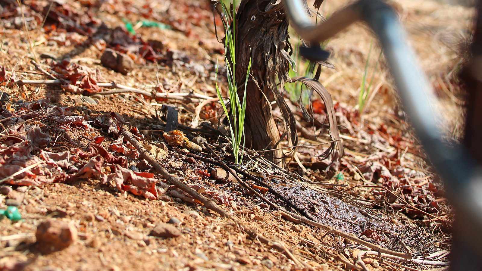
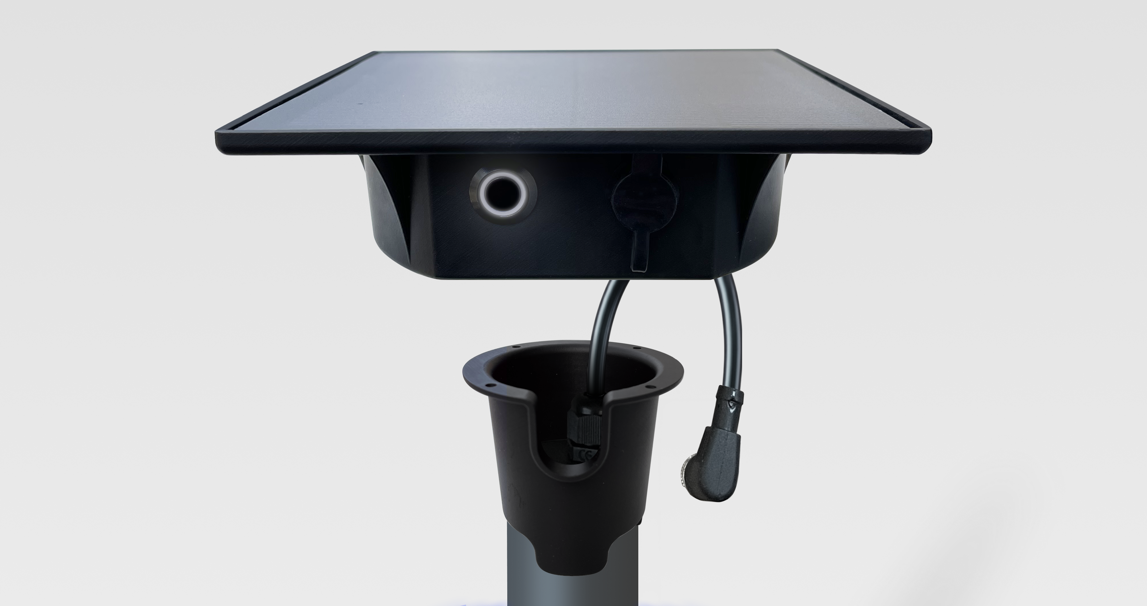
Should you refill the soil's available water before summer?

Oct 21, 2026 Akuasense 29 min read

Drip-irrigated vineyard row: the vines are aligned along the dripline, and a patch of moist soil spreads beneath an emitter. — Photo: Jessica Griffiths, USDA ARS (public domain).

During a heatwave, the water available to a crop in its root zone falls by the difference each day as soon as the irrigation system can no longer supply as much water as the crop evaporates. A soil profile filled to field capacity at the start of the heatwave therefore delays water stress, and the larger the total available water (TAW) of the soil, the longer the delay. Research shows a benefit in refilling the soil before summer only under certain conditions: an irrigation capacity well below the crop’s peak evapotranspiration, a dry soil at the end of winter, and an application limited to the root zone. On a soil that is already moist, much of the water applied drains below the roots.

During the heatwaves of summer 2026, the atmospheric demand for water often exceeded what irrigation systems could supply. Soil moisture then fell, even when irrigation was running at full capacity. Three quantities explain this: the amount of water the soil can release to the crop, the amount the crop and the soil evaporate each day, and the amount the irrigation system can supply each day. This article explains each of them, with sources, then examines what research says about refilling the soil before summer: preseason irrigation and an early start to the irrigation season. A calculator and three simulators let you apply these concepts to a field.

Terms used

mm of water: Depth of the layer of water spread over the soil surface. 1 mm of water equals 1 litre per square metre, or 10 m³ per hectare.
Horizon: Layer of soil with uniform characteristics. A soil generally consists of several horizons of different textures.
Root zone: Volume of soil in which the crop's roots are found. Its depth is the rooting depth.
Field capacity: Maximum moisture the soil retains once the drainage of water under gravity has become negligible.
Permanent wilting point: Moisture below which roots can no longer extract water from the soil.
TAW (total available water): Amount of water the soil can release to the crop: the water held between field capacity and the wilting point over the whole root zone, in mm of water, also called the soil's available water capacity. The remaining available water is the part of this water still present at a given time.
RAW (readily available water): Part of TAW that the crop extracts without reducing its transpiration.
Water stress: State of a crop that reduces its transpiration because it cannot extract enough water from the soil.
ETo: Reference evapotranspiration: the amount of water evapotranspired in one day by a well-watered reference grass surface, calculated with the FAO Penman-Monteith method, in mm of water per day. It expresses the climate's demand for water. In France it is often called ETP (évapotranspiration potentielle, potential evapotranspiration), a term FAO discourages because it has covered different definitions and formulas.
ETc: Evapotranspiration of a crop that is not short of water, in mm of water per day: ETc = Kc × ETo, where Kc is the crop coefficient.
Irrigation capacity: Maximum net amount of water the irrigation system can make available to the crop each day, after losses, in mm of water per day.
Heatwave: Period of temperatures well above normal for the time of year, lasting several consecutive days. Météo-France identifies one at national level when the national thermal indicator reaches or exceeds 25.3 °C and remains high for at least three days.¹

Key points

TAW depends on the texture, stone content and thickness of each horizon within the root zone. Calculated from the water contents published by FAO for a uniform soil without stones, it ranges, for example, from 30 to 66 mm of water for a sand whose root zone reaches 60 cm, and from 117 to 171 mm of water for a loam whose root zone reaches 90 cm.
During a heatwave, the ETc of a crop whose foliage fully covers the ground can reach or exceed 10 mm of water per day, depending on the species, its growth stage and the climate. When the irrigation capacity is lower than ETc, the crop draws the difference from the soil, and the remaining available water falls every day, even if the system is running at full capacity.
Without rain, the remaining available water recovers only once ETc falls back below the irrigation capacity, and only at the rate of the difference between the two.
A full RAW at the start of a heatwave delays the onset of water stress. As a first approximation, with a constant deficit and no rain, the number of days gained equals the RAW divided by the daily deficit: with a deficit of 2.5 mm of water per day, 10 days for a RAW of 25 mm, 30 days for a RAW of 75 mm. This delay is shorter when ETc is high, because RAW then shrinks.
Once the whole root zone has been brought back to field capacity, any additional water drains below the root zone and can carry away the nitrates it contains.
Refilling the soil before summer has shown a benefit only under certain conditions: an irrigation capacity well below peak ETc (for maize in Kansas, a gain at 2.5 mm of water per day, not at 5 mm), a dry soil at the end of winter and an application limited to the root zone. For vines, after a dry winter, an application during dormancy worked better than one at budburst. On a soil that is already moist, much of the water applied is lost.

Three figures, one mechanism: 8 mm supplied, 10.5 mm of ETc, 24 mm of RAW

One of the farmers who use our probes summed up his summer for us in three figures. During the heatwaves, the reference evapotranspiration (ETo) in his area reached 10 to 11 mm of water per day. His irrigation system, limited by the flow rate of his pump and by the water rotation, the schedule that sets the days or hours when each irrigator may draw water, could not supply more than 8 mm of water per day. The readily available water (RAW) of his fields is 20 to 25 mm of water. Although he irrigated at the full capacity of his system, soil moisture in his fields never returned to the level he was aiming for.

8 mm/day

Irrigation capacity

The maximum amount of water the irrigation system can supply to the crop each day.

10–11 mm/day

ETo

The atmospheric demand for water: the water evaporated each day by a well-watered reference grass surface.

20–25 mm

RAW

The soil water the crop extracts without reducing its transpiration.

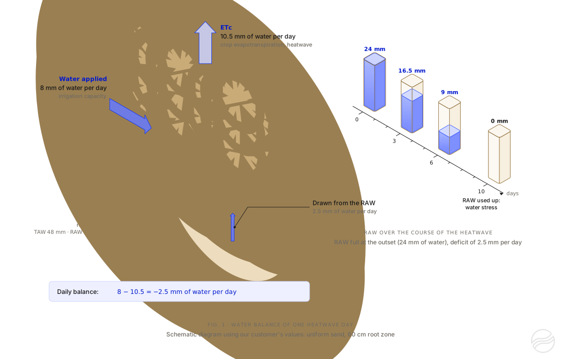
For a crop whose foliage fully covers the ground, ETc is of the same order as ETo; depending on the species and its growth stage, it may be lower or higher (part 3). Let us assume here that ETc equals ETo, that is, 10.5 mm of water per day, the middle of the range, and that the 8 mm applied are fully available to the crop. On each day of the heatwave, ETc then exceeds what the system supplies by 2.5 mm of water, and the remaining available water falls by the same amount. A RAW of 24 mm, full at the start of the heatwave, is used up in about 10 days (24 ÷ 2.5 = 9.6). Summer 2026 had three heatwaves, from 17 to 30 June, from 4 to 19 July and from 28 July to 19 August, 53 days in all; according to Météo-France, the French national meteorological service, it was the hottest summer recorded in France since measurements began in 1900².

Isometric diagram: a trellised vine under drip irrigation receives 8 mm of water per day and loses 10.5 mm through evapotranspiration; the missing 2.5 mm are drawn from the readily available water (RAW) of the 60 cm root zone. On the right, four reservoirs along a time axis show RAW at 24 mm of water on day 0, then 16.5 mm, 9 mm and 0 mm on day 10. The animation runs through the ten days: the soil dries out and, once RAW is used up, the vine goes into water stress, with drooping leaves and shrivelled bunches. — **Figure 1.** Simplified balance for one heatwave day in our customer’s field, with an assumed ETc of 10.5 mm of water per day and an application of 8 mm fully available to the crop, shown here by a vine as an example. The 2.5 mm of water missing each day are drawn from RAW: full at 24 mm at the outset, it is used up in about 10 days. On the right, RAW is shown as a reservoir: the water level represents the amount remaining, not where the water is in the soil. This calculation is refined in part 5.

This case is not isolated. For maize, Arvalis, the French applied research institute for arable crops, reports that daily ETo reached 10 mm of water at the peak of the heatwave of late June 2026, and that it “often exceeded the capacity of irrigation equipment (even under centre pivots)” (our translation)³. The following parts detail the three quantities involved: total available water, ETc and irrigation capacity.

Available water capacity (TAW) and RAW: the water the soil can release to the crop

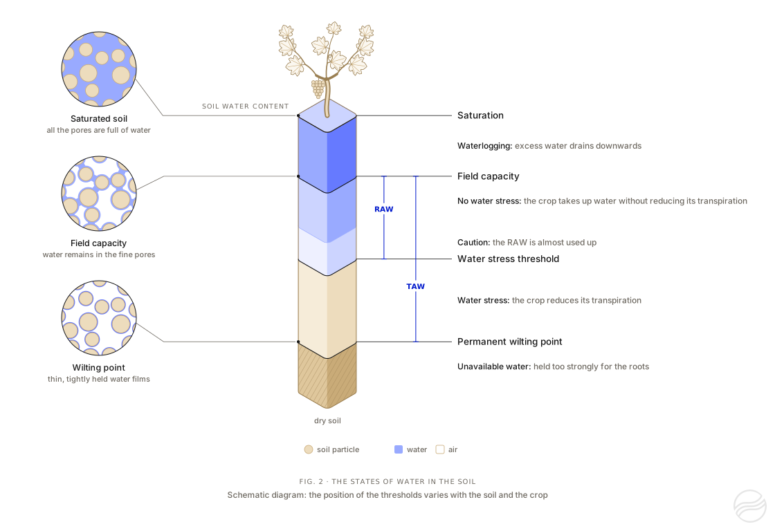
A soil consists of mineral and organic particles separated by voids, the pores. The water in these pores is not held everywhere with the same force. Several states are therefore distinguished, characterised by soil moisture, that is, the share of the soil’s volume occupied by water.

Saturation. When rain or irrigation fills all the pores, the soil is saturated. Water in the largest pores then drains downwards under gravity.
Field capacity. When this drainage becomes negligible, the remaining water is held by capillarity in the finest pores and around the particles. The moisture reached at this stage is field capacity: the maximum moisture the soil retains over time. Once the whole root zone is at field capacity, any additional water drains below it⁴.
Permanent wilting point. As roots take up water, the water that remains is held more and more strongly. At the permanent wilting point, roots can no longer extract it, and the plant wilts without recovering.

On the left, three magnified views of soil particles: saturated soil, field capacity and permanent wilting point. In the centre, a scale from dry soil to saturation, topped by a vine, with four thresholds: saturation, field capacity, water stress threshold and permanent wilting point. RAW runs from field capacity to the water stress threshold, TAW from field capacity to the wilting point. On the right, the corresponding states: waterlogging, no water stress, caution, water stress, unavailable water. The animation highlights each state in turn, and the vine responds: upright down to the caution zone, drooping leaves and shrivelled berries under water stress, leaves and bunch fallen to the ground below the wilting point. — **Figure 2.** The states of water in the soil. On the left, soil particles under a magnifying glass: at saturation, water fills all the pores; at field capacity, it occupies only the finest pores; at the wilting point, only thin films remain around the particles. In the centre, the soil water content, from dry soil (beige) to saturation (blue), and the four thresholds that separate the states of water for the crop. The vine planted on top of the scale represents the crop; the animation shows how it responds to each state of the water. Schematic diagram: the position of the thresholds varies with the soil and the crop.

Total available water (TAW), often called the soil’s available water capacity, is the water held between field capacity and the wilting point over the whole root zone⁴. Rooting depth depends on the species, the variety or rootstock, the age of the plants, the irrigation method and the obstacles the roots encounter: a compacted horizon, bedrock, a water table.

Calculating a soil’s available water capacity

The amount of water a soil can store and release to plants is calculated horizon by horizon, then added up⁵. For a given crop, only the horizons its roots reach are counted:

\mathrm{TAW} = \sum_{\text{horizons}} \left( \theta_{FC} - \theta_{WP} \right) \times d

$\mathrm{TAW}$ : total available water, in mm of water, summed over each horizon of the root zone

$\theta_{FC}$ , $\theta_{WP}$ : volumetric water content at field capacity and at the wilting point, in m³ of water per m³ of soil

$d$ : horizon thickness, in mm

example: a 30 cm loam horizon ( $\theta_{FC} = 0.30;\ \theta_{WP} = 0.15$ ) over a 30 cm sand horizon ( $\theta_{FC} = 0.15;\ \theta_{WP} = 0.07$ )

TAW over 60 cm: $0.15 \times 300 + 0.08 \times 300 = 45 + 24 = 69$ mm of water

The water contents $\theta_{FC}$ and $\theta_{WP}$ depend on the texture of the horizon, that is, its proportions of sand, silt and clay, but also on its organic matter content, its structure and its degree of compaction. Rock fragments (stones and gravel) reduce the volume of fine earth that holds water; how to account for them precisely is still the subject of research⁵. The following table gives orders of magnitude for a horizon of uniform texture, without stones.

Horizon texture (USDA class)	Available water capacity (mm of water per cm of soil)	TAW over 30 cm (mm of water)	over 60 cm	over 90 cm
Sand	0.5–1.1	15–33	30–66	45–99
Sandy loam	1.1–1.5	33–45	66–90	99–135
Loam, silt loam	1.3–1.9	39–57	78–114	117–171
Clay	1.2–2.0	36–60	72–120	108–180

Values calculated from the water contents at field capacity and at the wilting point published by FAO (Table 19 of FAO-56)⁴. FAO uses the US (USDA) soil texture classification, whose classes do not exactly match those of the texture triangle used in France. Compaction changes these values: the Drôme Chamber of Agriculture, for example, uses 1 mm of water per cm of soil for an uncompacted sand and 0.7 mm for a compacted sand⁶.

When a soil analysis gives the proportions of sand, silt and clay and the organic matter content, $\theta_{FC}$ and $\theta_{WP}$ can be estimated with pedotransfer functions. Those of Saxton and Rawls, developed from soils in the United States, are the ones the hub uses⁷. In France, the reference values for each class of the French (Aisne) texture triangle are those of Bruand, Duval and Cousin. They were measured on undisturbed soil clods and distinguish the tilled horizon from the deeper horizons, but they do not cover calcareous horizons⁸. The two methods do not use the same definition of field capacity: the water content at a tension of 33 kPa for Saxton and Rawls, and of 10 kPa (pF 2) for the French references. The latter gives a higher field capacity, and therefore a larger TAW. In the laboratory, the available water of a horizon is measured from its water content at pF 2, determined on undisturbed clods, and at pF 4.2, the wilting point⁹.

Stones and gravel occupy part of the soil volume. By convention, they are treated as inert, and the available water of the horizon is reduced in proportion to their volume; Arvalis considers that they can be ignored below 10% of the volume⁹. Yet not all of them are inert. According to the values used by Arvalis, one centimetre of stones holds about 0.2 mm of water for flint, 1 mm for limestone and 2.3 mm for chalk⁹. For a loamy clay horizon containing 30% stones, Tetegan and colleagues calculated that ignoring this water underestimates the available water by 5% with chert and by 33% with chalk¹⁰.

\begin{aligned} \mathrm{AW}_{h} = \bigl[\, & \mathrm{AWC}_{fe} \times (100 - \mathrm{RF}) \\ & + c \times \mathrm{RF} \,\bigr] \times \frac{d}{100} \end{aligned}

$\mathrm{AW}_{h}$ : available water of the horizon, in mm of water

$\mathrm{AWC}_{fe}$ : available water capacity of the fine earth, in mm of water per cm

$c$ : water held by the stones, in mm of water per cm

$\mathrm{RF}$ : share of the horizon volume occupied by rock fragments (stones and gravel), in %

$d$ : horizon thickness, in cm

example: a 40 cm horizon holding 1.5 mm of water per cm of fine earth, with 30% of limestone stones holding 1 mm of water per cm: $(1.5 \times 70 + 1 \times 30) \times 40 \div 100 = 54$ mm of water, compared with 42 mm if the stones are treated as inert

Clay-limestone soils, the French argilo-calcaires, illustrate these limits. The term denotes a type of soil rather than a texture class, and the available water of these soils depends first on the depth to the limestone bedrock and on their stone content. At the Arvalis experimental farm at Boigneville (Essonne), TAW of a shallow clay-limestone soil, which contains about 10% stones in its top 40 cm, above a highly calcareous horizon, is around 55 mm of water; that of a neighbouring clay loam, where hard limestone appears only below 120 cm, is around 120 mm¹¹. In Poitou-Charentes, the regional soil reference system uses, for calculating nitrogen fertilisation, a TAW of 60 to 80 mm of water for shallow groie soils, 80 to 110 mm for medium groies and 110 to 130 mm for deep groies¹². In Petite Beauce, TAW of two stony soils over hard limestone, calculated from the water retention measured in the laboratory on the fine earth and on the stones, is 54 mm of water for 50 cm of soil, with 22% stones at the surface, and 109 mm for 80 cm of soil, with 34% stones at the surface and 57% at 70 cm¹³. Bedrock is not always a limit for roots: Arvalis points out that fractured hard rock can be explored by roots⁹. For these soils, texture tables give only an order of magnitude; measurements by horizon, or monitoring soil moisture at several depths, show how much water the crop actually uses.

Tool 1: Soil available water capacity (TAW) calculator

Tool page

Estimate how much water your soil can supply to your crop (TAW and RAW), horizon by horizon.

Examples

Your crop

Crop

Depletion fraction p of 0.50, the value FAO cites as commonly used.

Rooting depth 60 cm
Set the rooting depth you observe in your field.
Your soil, horizon by horizon

Describe each horizon, from the surface downwards: one tab per horizon. The profile is redrawn after each change.

Available water held by each horizon
The result

Run the simulation to calculate the result with your settings.

Total available water (TAW)
69mm of water
over 60 cm of root zone, i.e. 690 m³/ha
Readily available water (RAW)
35mm of water
depletion fraction p of 0.50 for this crop
RAW during a heatwave
21mm of water
for an ETc of 10 mm of water per day (p of 0.30)
readily available: 35 mmharder to extract: 35 mm
Without rain or irrigation, a crop with an ETc of 5 mm of water per day uses up this RAW in about 7 days.

Indicative calculation, horizon by horizon. Water contents are estimated from the texture class or from the particle-size distribution, depending on the method chosen: Saxton and Rawls⁷, with the US (USDA) texture classes, or Bruand, Duval and Cousin⁸, with the classes of the French (Aisne) texture triangle. The water held by stones follows the values used by Arvalis⁹. RAW is calculated with the depletion fraction p of the chosen crop, taken from FAO-56 or from its 2021 update, or used by the hub^4,^14,¹⁵. Only a measurement by horizon gives the available water of a given field.

Detailed instructions, how to read the result and reference values: Calculate the available water capacity of a soil.

Not all the water in TAW is equally easy to extract. As long as soil moisture stays above a threshold specific to the crop, roots take up water without the crop reducing its transpiration: this part of TAW is RAW. Below this threshold, the remaining water is held more strongly; the crop can no longer extract as much as its ETc and partially closes its stomata, the leaf pores through which it transpires. This is water stress. The part of TAW below this threshold, TAW − RAW, can still be extracted, but only with difficulty.

RAW is not a fixed proportion of TAW. It depends on the crop, and sometimes on the variety: root distribution, tolerance to water shortage. It also depends on the current ETc (see the box below) and on the soil horizons. For each crop, FAO publishes a reference depletion fraction, denoted p, valid for an ETc of about 5 mm of water per day: for example, 0.40 for tomato or almond, 0.55 for grain maize and 0.65 for olive. The hub, like this article, uses these fractions. FAO specifies that this fraction ranges from 0.30 for shallow-rooted plants whose ETc exceeds 8 mm of water per day to 0.70 for deep-rooted plants whose ETc is below 3 mm of water per day⁴. Irrigation scheduling tools often use a single fraction, for simplicity. Arvalis states that RAW represents 40 to 80% of TAW depending on soil depth, that is, the thickness of soil above bedrock or above a horizon that roots do not cross, and on the crops grown¹⁶.

With the fraction of 0.5 that FAO cites as commonly used, a RAW of 20 to 25 mm of water corresponds to a TAW of 40 to 50 mm: for example, a sand holding 0.8 mm of water per cm of soil, explored by roots over 50 to 60 cm, or a loam holding 1.7 mm of water per cm of soil, explored over 25 to 30 cm. By comparison, a uniform loam explored by roots over one metre can offer a TAW of 130 to 190 mm of water.

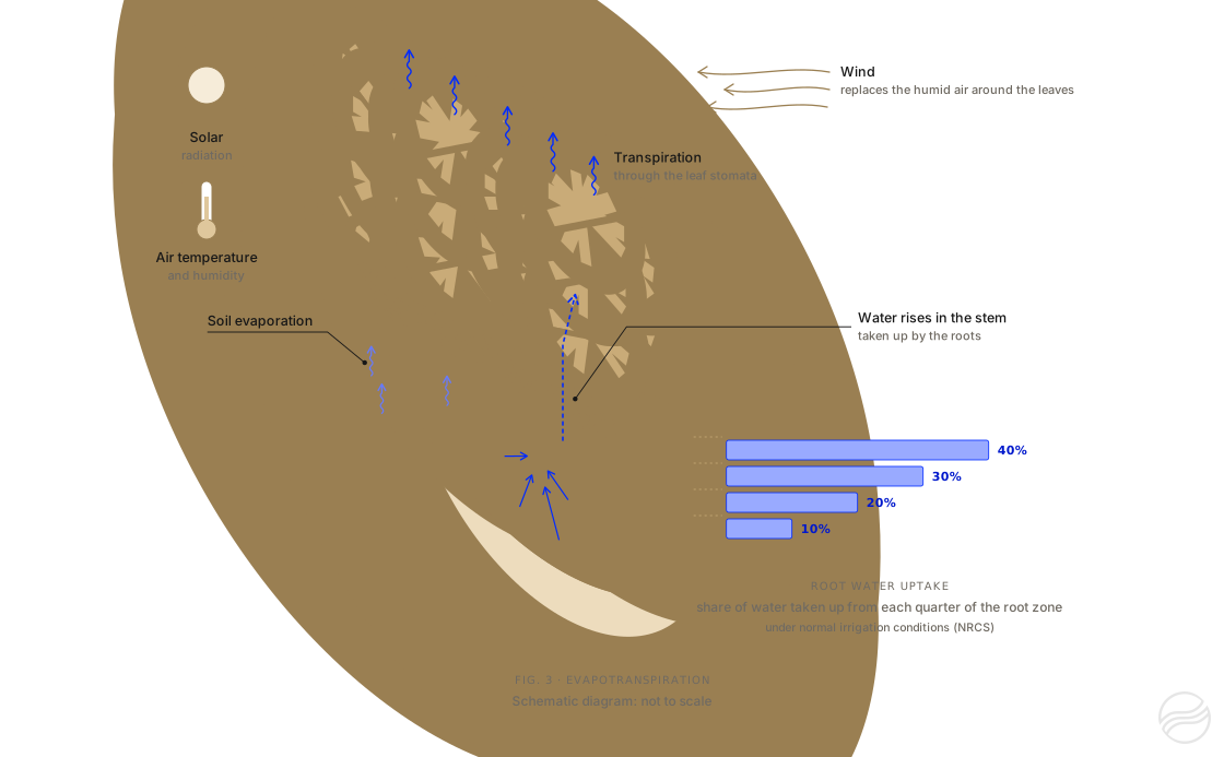
Crop evapotranspiration (ETo, Kc and ETc)

Nearly all the water taken up by the roots passes through the plant and evaporates through the stomata: this is transpiration⁴. Added to this is the evaporation of water directly from the soil surface. The sum of the two is evapotranspiration.

Evapotranspiration depends on the climate: solar radiation, temperature, air humidity and wind. To measure this effect independently of the crop, the evapotranspiration of a reference surface is calculated: a grass 12 cm tall, completely covering the ground, actively growing and well supplied with water. This is the reference evapotranspiration, ETo⁴. For arid and semi-arid temperate regions, FAO puts its average values at 6 to 9 mm of water per day when the mean daily temperature exceeds 30 °C⁴. Peak values calculated during heatwaves are higher: 10 mm of water per day in late June 2026, according to Arvalis³.

Isometric diagram: a trellised vine on a block of soil in cross-section. Radiation, temperature, air humidity and wind draw water from the soil through the plant: the roots take it up, it rises in the stem and evaporates through the leaves; part of it evaporates directly from the soil. On the right, the share of water taken up from each quarter of the root zone: 40, 30, 20 and 10%. The animation moves the water from the soil to the air, taken up mostly from the upper quarter of the root zone; during a heat spike, the whole flow speeds up. — **Figure 3.** Radiation, temperature, air humidity and wind drive evapotranspiration: water taken up by the roots rises through the plant and evaporates through the leaves. Under normal irrigation conditions, roots take up about 40% of their water from the upper quarter of the root zone and 10% from the lowest quarter, according to the Natural Resources Conservation Service of the US Department of Agriculture¹⁷; this distribution varies with the crop, the soil and the irrigation method. The crop is shown as a trellised vine. Schematic diagram: not to scale.

ETc is obtained by multiplying ETo by the crop coefficient Kc⁴:

\mathrm{ETc} = \mathrm{Kc} \times \mathrm{ETo}

example: grain maize at mid-season, $\mathrm{Kc} = 1.20$ ¹⁴; $\mathrm{ETo} = 10.5$ mm of water per day; $\mathrm{ETc} = 12.6$ mm of water per day

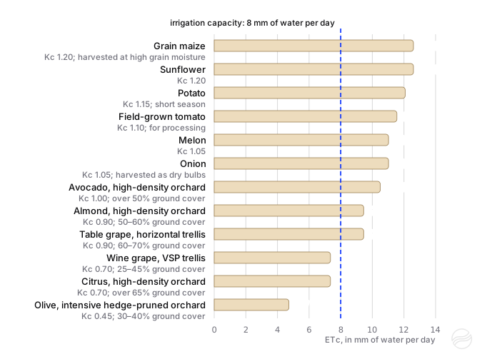
Kc depends on the species, its growth stage and the fraction of the ground covered by foliage. It also varies with the variety, planting density, crop management (pruning, inter-row cover crop) and climate: in 1998, FAO published reference values for a sub-humid climate, with a method for adjusting them to dry, windy climates⁴. These values were updated in 2021 on the basis of the measurements published since: for field crops and vegetable crops by Pereira and colleagues^14,¹⁵, for fruit trees and vines by Rallo and colleagues¹⁸. For the latter, Kc is given by planting density and ground cover class rather than by species. These updated values are the ones the hub and this article use. With these values and an ETo of 10.5 mm of water per day, an irrigation capacity of 8 mm of water per day does not cover the mid-season ETc of any of the field or vegetable crops in figure 4 (maize, sunflower, potato, tomato, melon, onion), nor that of almond, table grapes or avocado; it does cover that of a wine grape vineyard, an olive orchard or a citrus orchard. For maize, Arvalis gives a consistent order of magnitude: with an ETo of 7 mm of water per day, the ETc of maize at flowering reaches 9 mm of water per day¹⁹.

Bar chart: mid-season ETc of 12 crops for an ETo of 10.5 mm of water per day, compared with an irrigation capacity of 8 mm of water per day. Grain maize: 12.6 mm; Sunflower: 12.6 mm; Potato: 12.1 mm; Field-grown tomato: 11.6 mm; Melon: 11.0 mm; Onion: 11.0 mm; Avocado, high-density orchard: 10.5 mm; Almond, high-density orchard: 9.5 mm; Table grape, horizontal trellis: 9.5 mm; Wine grape, VSP trellis: 7.4 mm; Citrus, high-density orchard: 7.4 mm; Olive, intensive hedge-pruned orchard: 4.7 mm. — **Figure 4.** Mid-season ETc of a few crops for an ETo of 10.5 mm of water per day, calculated with the standard Kc values updated in 2021, without climatic adjustment, and compared with an irrigation capacity of 8 mm of water per day. For fruit trees and vines, Kc depends on planting density and on ground cover, that is, the fraction of the ground covered by foliage: the class used is shown under each of these crops. Actual values also depend on the variety, crop management and local climate^14,^15,¹⁸.

When water becomes hard to extract, the crop partially closes its stomata. It thereby limits its water losses, but at the same time reduces its photosynthesis and growth. FAO stresses that flowering and yield formation are stages sensitive to water shortage, whereas stress during the vegetative or ripening phase generally has a more limited impact²⁰. A water shortage during these sensitive stages therefore weighs more heavily on yield.

How to calculate the irrigation capacity of a system

Between the water source and the roots, every component of the irrigation system can limit the amount of water applied. The amount of water pumped per day, divided by the irrigated area, is the gross application. Part of this water does not reach the root zone: evaporation, wind drift, runoff or deep percolation below the root zone. The share of the pumped water that remains available to the crop is the application efficiency. The irrigation capacity is the maximum gross application multiplied by the application efficiency.

Isometric diagram: reservoir, electric centrifugal pump, disc filter with pressure gauges, solenoid valve and controller, then a dripline hung from the bottom wire of a trellised vine row. The soil cross-section, hatched by horizon, shows the water applied beneath the emitters and the Akuasense probe placed near a vine, which measures soil moisture and temperature every 15 cm; its gateway sends the readings to the hub over 4G. Legend with the standard symbol of each component. The animation shows one irrigation, then the soil drying: water flows through the pipes, a drop falls from each emitter, and the curve in the hub follows the soil moisture. 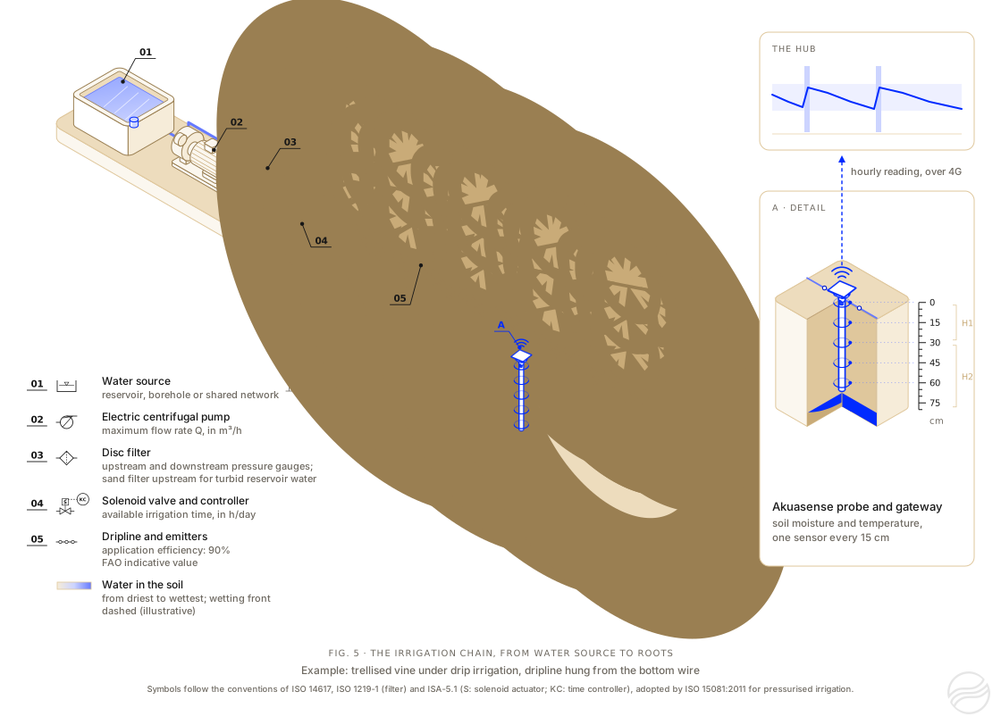— **Figure 5.** A drip irrigation system, from the water source to the roots: a reservoir, an electric pump, a disc filter, a solenoid valve operated by a controller and a dripline along a vine row. The probe measures soil moisture at several depths; the gateway sends its readings over 4G every hour. The legend symbols follow the conventions of ISO 1219-1, ISO 14617 and ISA-5.1.

G = \frac{Q \times t}{10 \times A}

$G$ : maximum gross application, in mm of water per day

$Q$ : pump flow rate, in m³/h; $t$ : irrigation time available, in h/day; $A$ : irrigated area, in ha

the factor 10 comes from the fact that 1 mm of water over 1 ha represents 10 m³

C = G \times E

$C$ : irrigation capacity, in mm of water per day; $E$ : application efficiency

example: $40 \times 20 \div (10 \times 9) = 8.9$ mm of water pumped per day (40 m³/h, 20 h/day, 9 ha); with an application efficiency of 90%, 8.0 mm of water per day remain available to the crop

Four quantities therefore set the gross application: the pump flow rate, the irrigation time available each day, the number of days of access to water and the irrigated area.

Tool 2: Irrigation system capacity calculator

Tool page

Compare the water your irrigation system delivers each day with your crop's peak demand, then convert a depth into an irrigation time or, for a hose reel, into a travel speed.

Examples

Your system
The calculation covers one water supply point (pump, hydrant or canal) and the area it irrigates with a single irrigation method. The fields to fill in depend on the irrigation method chosen.
The calculator assumes similar blocks: same irrigation method, same equipment, same area, same irrigation time. If that is not the case, run one calculation per block:
1. in step 1, choose the irrigation method of that block, then enter the flow rate it receives and its own area or, if its irrigation method allows, its emitters or sprinklers, with “Number of blocks” set to 1;
2. in step 2, enter the number of hours that block receives water each day;
3. copy the calculation link to keep it, then move on to the next block.
Example: a pump runs 20 hours a day for two blocks, tomatoes irrigated for 12 hours and melons for 8 hours. Two calculations are then needed, one with 12 hours, the other with 8 hours.

For several independent pumps, run one calculation per pump. If several pumps supply the same network, add their flow rates together.
Irrigation method

Application efficiency 90%
Preset value for this irrigation method: nothing needs to be entered. FAO uses 90%; Irmak and colleagues give 85 to 95% for a well-designed and well-managed system.

Calculation basis

Both options describe the same system: choose one and fill in only its fields.

With this irrigation method, the calculation is based on the pump flow rate and the irrigated area.

Flow rate of the pump or hydrant

The flow actually delivered during irrigation, not the maximum flow quoted for the pump.

Irrigated area

The whole area supplied by this water supply point, all blocks included: 9 ha irrigated in three 3 ha blocks counts as 9 ha.

40 m³/h over 9 ha 0.44 mm of water per hour, over the whole area
Average over the whole area: with this method, blocks do not need to be entered. 1 mm of water over 1 ha is 10 m³.
Irrigation time

Irrigation time available per day 20 h
Excluding breakdowns, equipment moves and abstraction bans: a ban from 11:00 to 18:00 removes 7 hours.

Days of access to water per week 7 / 7
Water rotation or ban days: a two-day weekly ban leaves 5 days a week.
Crop requirement

The crop's peak ETc

Peak ETc 10.5 mm/day
The water the crop uses each day at the peak.

The field's RAW 24 mm

To find for how many days the soil's reserve can make up the shortfall. Calculate a soil's RAW
Result

Run the simulation to calculate the result with your settings.

Gross application
8.9mm/day
every day, water pumped divided by the area
Irrigation capacity
8.0mm/day
after losses (90% application efficiency), i.e. 80 m³/ha/day
Share of ETc covered
76%
ETc of 10.5 mm/day: deficit of 2.5 mm of water per day
One irrigation dayAfter losses: irrigation capacity
Water the crop draws from the soil's reserve each day
On each peak day, the crop draws 2.5 mm of water from the soil's reserve: a full RAW of 24 mm is used up in about 10 days. The crop then reduces its transpiration.
To cover this ETc, irrigation would have to run 26 h a day, which is more than 24 h, or the pump would have to deliver 53 m³/h for 20 h.
Water pumped: 89 m³/ha/day, i.e. a continuous flow of 1.03 L/s/ha.
Set one irrigation

For the system described in step 1: the irrigation time that gives a depth, or the depth that a time gives.

What you know

Depth to apply

Gross depth: the water the system delivers, in mm over the whole area, before losses.

Blocks irrigated one after another
Similar blocks, as in step 1. Enter 1 if the whole area is irrigated at the same time.

Irrigation time
22 h 30min
10 mm at 0.44 mm of water per hour
The whole area
1.1irrigation days
22 h 30 min, at 20 h a day
Net depth
9.0mm
after losses (90% application efficiency)
This irrigation needs 22 h 30 min, more than the 20 h of irrigation available per day (step 2).
10 mm ÷ 0.44 mm/h → 22 h 30 min.

Indicative application efficiencies: 90% for drip irrigation and 75% for sprinkler irrigation according to FAO²¹; Irmak and colleagues give a “potential” range for each system, that of a well-designed and well-managed system²². In the field, efficiency depends on the condition of the equipment, wind, slope and irrigation management.

Detailed instructions, how to read the result and reference values: Calculate the capacity of an irrigation system.

Two factors reduce the amount of water that actually reaches the crop.

Water rotations. In a shared irrigation network, the water supplier may impose a rotation to share the water between irrigators²³. During droughts, orders issued by the prefect, the State’s representative in each French département, may also restrict irrigation on certain days or at certain hours: in 2023, for example, the alert level in Gironde imposed either a ban on agricultural abstraction two days a week or a 30% reduction in volume or time²⁴. A system that applies 8 mm of water on the days it runs, but only 5 days out of 7, applies on average 5.7 mm of water per day.
Application efficiency. With an efficiency of 90%, 8.9 mm of water pumped leave only 8.0 mm available to the crop.

By comparison, in the Adour basin, in 2009, authorised abstraction volumes were converted into irrigable areas on the basis of a theoretical unit requirement of 0.7 L/s/ha on free-draining soils (sands, alluvium) and 0.6 L/s/ha on heavy soils (molasse)²⁵, that is, 6.0 and 5.2 mm of water pumped per day, continuously. During the 2026 heatwaves, ETo exceeded these values, as it exceeded our customer’s 8 mm of water per day.

Why the soil’s remaining available water falls during a heatwave

The water balance of a field compares, day after day, the water entering and leaving the root zone: the change in remaining available water equals rain and irrigation, minus crop evapotranspiration and deep percolation below the root zone; runoff and capillary rise from a water table are ignored here⁴. Without rain, the balance comes down to the difference between irrigation and evapotranspiration. As Fereres and Soriano put it, when irrigation is less than evapotranspiration, the crop draws on the soil water reserves to make up the deficit²⁶. Three phases then follow.

During the heatwave, ETc exceeds the irrigation capacity, and the remaining available water falls each day by the difference. As the system is already running at full capacity, no change to irrigation can prevent this fall.
When the remaining available water falls below the water stress threshold, the crop reduces its transpiration: its actual evapotranspiration becomes lower than its ETc. The remaining available water then levels off, not because irrigation is sufficient, but because the crop’s actual evapotranspiration has fallen to the water the system supplies. Stable soil moisture during a heatwave therefore does not mean that the crop is well supplied with water.
After the heatwave, ETc falls, for example to 6 mm of water per day. Without rain, the remaining available water recovers only at the rate of the difference between irrigation capacity and ETc: 8 − 6 = 2 mm of water per day. It therefore takes 10 days to rebuild a RAW of 20 mm. In 2026, the intervals between the heatwaves lasted only 3 days, from 1 to 3 July, and 8 days, from 20 to 27 July².

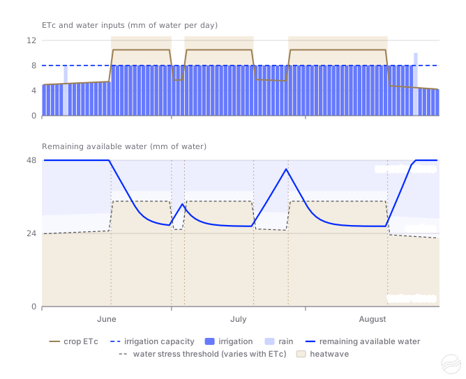
Figure 6 applies this balance, day by day, to a field whose RAW is close to our customer’s. The remaining available water recovers only between heatwaves, by about 2 mm of water per day: the 3 days in early July are not enough, while the 8 days in late July bring the soil almost back to field capacity just before the third heatwave. During each heatwave, the remaining available water falls below the water stress threshold, then levels off there. This mechanism is consistent with what our customer observed.

Figure 6. Simulated daily water balance, from June to August, on the dates of the 2026 heatwaves. Assumptions, chosen to illustrate the mechanism: uniform sand without stones holding 0.8 mm of water per cm of soil, 60 cm root zone (TAW of 48 mm of water, reference RAW of 24 mm), crop with full ground cover (Kc of 1.0), ETo held at 10.5 mm of water per day for the whole duration of the heatwaves (a high assumption: Arvalis reports 10 mm at the peak), irrigation capacity of 8 mm of water per day used to the full, soil at field capacity on 1 June. The dotted line marks the water stress threshold; it rises during the heatwaves, as explained in the box in part 2. FAO water balance model⁴, for teaching purposes. Hover over the chart to read the values.

Refilling the soil profile before summer: when is it worthwhile?

Another farmer gave us this advice: start irrigating earlier, even before the season, to fill the soil profile and go into the summer heatwaves with a full root zone, rather than trying to make up a deficit afterwards. Two practices are involved: preseason irrigation, carried out before sowing or before growth resumes in spring, and an early start to the irrigation season. They rest on the same physical principle: when the irrigation capacity no longer covers ETc, the remaining available water is the only water the crop has. In spring, ETc remains lower than the irrigation capacity: water stored in the root zone at that time can be used during the peak period, provided it stays there. Research shows that part of it is lost, and that the benefit depends on the irrigation capacity, on soil moisture at the end of winter and on the crop.

What research shows on preseason irrigation

Preseason irrigation has been studied in detail in the US Great Plains, mainly for maize, on very deep silt loams irrigated by systems with a gross capacity of 2.5 to 5 mm of water per day. These results do not transfer directly to other soils, crops or climates, but they shed light on the mechanisms involved.

At Kansas State University, Schlegel and colleagues measured, on a deep silt loam in Kansas, the storage efficiency of preseason irrigation: the increase in soil water between the previous harvest and maize emergence, divided by the 75 mm of water applied in April. It reached 82% for plots irrigated in season at 2.5 mm of water per day, 62% at 3.8 mm and only 27% at 5 mm per day, because the latter ended the previous season with a wetter soil. Over four years, two of them dry, preseason irrigation increased maize yield by 1 t/ha on average, about 9%; the authors nevertheless consider that it is probably not justified when the gross irrigation capacity reaches 5 mm of water per day or more²⁷.
A soil water balance modelling study carried out at Kansas State University shows that the share of water stored depends on soil moisture at the time of application: it reaches 90 to 95% for a spring application on a very dry soil, and decreases rapidly on a wetter soil, especially when the remaining available water exceeds 60% of TAW²⁸.
In Texas, a cotton study cited by Lamm and colleagues measured losses of 45 to 70% of the water applied before sowing by low-capacity systems, over the 30 to 45 days preceding sowing²⁹.
A modelling study of maize at the same Kansas site, with 29 years of weather data, concludes that with a gross irrigation capacity of 2.5 mm of water per day or less, 75 to 100 mm of water applied before sowing increase median yield by 10 to 17% in years of normal rainfall. Citing the reference review by Musick and Lamm, it points out that the decision must be based on knowledge of soil water and of the local rainfall pattern³⁰.
For walnut and prune orchards in the Sacramento Valley, California, University of California farm advisors recommended, after a dry February, applying 75 to 100 mm of water in several applications before the season. This amount leaves room in the soil to store the rain to come³¹.

Vines and orchards: winter, budburst or later?

In Australia, in the Barossa, SARDI and CSIRO researchers simulated dry winters on Shiraz by excluding rain from May to August for three seasons. Cutting winter rainfall to a third of the average reduced yield by 20 to 40%. Winter irrigation by micro-sprinklers gave results close to the control; filling the soil at budburst did not offset the yield loss, increased canopy growth and degraded the composition of the grapes and wines^32,³³.
In Spain, in Ribera del Duero, on Tempranillo trained as cordon de Royat on a deep sandy loam, gravelly below 50 cm, a recharge of 110 to 136 mm of water by drip before budburst added nothing to summer deficit irrigation: 8.0 t/ha with the recharge, 7.9 t/ha without, on average from 2021 to 2023. Without summer irrigation, the recharge alone gave about 3.4 t/ha³⁴.
In California, on walnuts on a deep silt loam to fine sandy loam, delaying the start of irrigation on the basis of stem water potential, measured on the tree, saved about 250 mm of water per season (710 mm versus 965 mm) without yield loss, except for a 10% drop one year at the latest threshold. The authors consider that a soil kept too full in spring can cause more problems than it solves³⁵.

What French references say about starting irrigation

The French references we found deal with starting irrigation in season, not with refilling the soil before summer; none of them recommends filling the soil profile before summer, and we found no French trial on Mediterranean perennial crops. For maize, Arvalis considered irrigation unnecessary before the 10-visible-leaf stage, except for difficult emergence or to make better use of nitrogen, and limited the first application to 20 to 25 mm of water to avoid drainage and runoff³⁶. From that stage on, two references stress starting without delay. The irrigation bulletin of the Ain plain, written with Arvalis and the Chamber of Agriculture, aims for a start at around 10 leaves, so that the last field of the irrigation round is irrigated at 12 leaves without stress: “A late start can only be made up for by a significant rainfall event!” (our translation)³⁷. When early restrictions are feared, Arvalis’s advice is to “use the water available from the very start of the irrigation period” and to “preserve the soil water reserve as much as possible” (our translation)³⁸. For wheat, a technical bulletin from Ouest Occitanie in spring 2020 based the start of irrigation on TAW, later in deep soils, noting that “irrigation that is too early and too abundant leads to excessive vegetative growth, which results in increased transpiration” (our translation)³⁹. For vines, the Var Chamber of Agriculture notes that early in the season, water is “often drawn from the soils’ winter reserves”, and that irrigation “generally starts around mid-June” (our translation)⁴⁰.

What a full RAW provides

As a first approximation, with a constant deficit and no rain, the number of days by which a full RAW delays water stress equals RAW divided by the daily deficit, that is, by the difference between ETc and irrigation capacity. With an irrigation capacity of 8 mm of water per day and an ETc of 10.5 mm of water per day, the deficit is 2.5 mm of water per day.

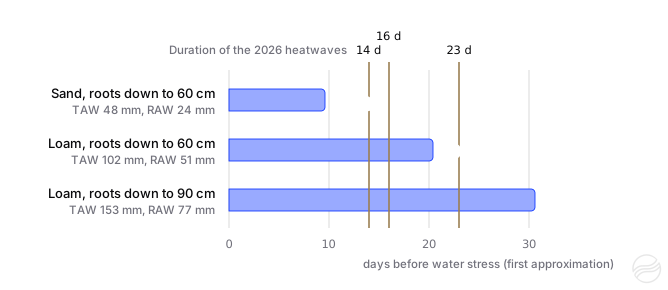
Bar chart: days before water stress, as a first approximation, for a full RAW at the start of a heatwave and a constant deficit of 2.5 mm of water per day. Sand, roots down to 60 cm: 10 days; Loam, roots down to 60 cm: 20 days; Loam, roots down to 90 cm: 31 days; Duration of the 2026 heatwaves: 14 d, 16 d, 23 d. — **Figure 7.** Number of days before water stress sets in, calculated as a first approximation for a full RAW at the start of a heatwave and a constant deficit of 2.5 mm of water per day, compared with the duration of the three heatwaves of summer 2026. Assumptions: uniform horizons without stones, holding 0.8 mm of water per cm of soil for the sand and 1.7 mm for the loam (values chosen within the ranges of the table in part 2), RAW equal to half of TAW. This calculation takes into account neither the reduction in RAW when ETc is high, nor days of respite.

This calculation gives 10 days for the sand explored over 60 cm and 31 days for the loam explored over 90 cm. The simulation, which takes the reduction in RAW into account, gives less. For the sand (figure 6), water stress appears from the 7th day of the first heatwave. For the loam irrigated from 1 April, the first heatwave passes without water stress, and stress appears on 10 July, the 7th day of the second heatwave (tool 4). A full soil profile therefore helps most where RAW is highest: 77 mm of water for this loam explored over 90 cm, compared with 24 mm for the sand explored over 60 cm.

Limitations

The soil does not hold water beyond field capacity. Once the whole root zone is at field capacity, any additional water drains below it. Arvalis points out the risks of excess water: loss of the water the soil cannot store; nitrate leaching, that is, nitrogen carried away as nitrates by the draining water; oxygen deprivation of the roots in waterlogged soils, that is, soils saturated with water temporarily or permanently³⁸.
A soil kept full can no longer store rain. In spring, not filling the soil profile completely leaves room to store the rain to come³¹.
Early, frequent applications can limit deep rooting. On maize, the Tarn Chamber of Agriculture warns: “Watering too early will also lead to poor deep root development if the available water remains in the upper part of the soil” (our translation)⁴¹. And the amount of water accessible to the crop increases with rooting depth.
Water must be available. Shared networks and abstraction licences do not always allow irrigation out of season.

In summary, studies show a benefit in refilling the soil before summer only under certain conditions: an irrigation capacity well below peak ETc, a dry soil at the end of winter, a high TAW and an application limited to the root zone, which leaves room for rain. For vines, an application during dormancy worked better than one at budburst. All these sources make the decision depend on knowledge of soil water.

Filling the soil profile therefore means wetting the soil down to the crop’s rooting depth, without going beyond it, when the irrigation capacity exceeds ETc. This requires knowing how far down the water goes.

Tool 3: How far down does the water go?

Estimate how deep an irrigation wets the soil, depending on its texture and moisture beforehand.

Soil texture (uniform, without stones)

Remaining available water before the application, as a share of TAW

Crop rooting depth

Water applied

Run the simulation to calculate the result with your settings.

Simplified model: each soil layer must reach field capacity before water moves on to the next. The wetting front is the boundary between the soil wetted by the application and the drier soil below. In the field, it is more diffuse; the infiltration rate varies from one horizon to another and, under drip irrigation, water also spreads sideways depending on the texture.

Seasonal soil water balance simulator

The simulator below applies the FAO water balance day by day, from 1 April to 30 September, on the dates of the three heatwaves of 2026. It lets you vary soil texture, rooting depth, crop, irrigation capacity, ETo during the heatwaves and the irrigation start date. It illustrates the effect of each of these factors; its climatic assumptions are illustrative, and it does not predict the behaviour of a real field.

Tool 4: Soil water balance simulator

Follow the soil's water reserve day by day over a season, and the crop's water stress.

Examples

Soil texture (uniform, without stones)

Rooting depth

Crop (mid-season Kc)

Irrigation capacity

ETo during heatwaves

Irrigation start

Remaining available water on 1 April

Calculated available water

Run the simulation to calculate the result with your settings.

Days of water stress

Unmet ETc

Irrigation applied

Rain drained below the root zone

View monthly data

Assumptions: uniform soil without stones; ETo outside the heatwaves from 3.4 mm of water per day in mid-April to 5.9 mm in mid-July (illustrative Mediterranean climate); rainfall of 59 mm of water in April, 36 in May, 8 in June, 0 in July, 10 in August and 40 in September; heatwaves on the 2026 dates, with a constant ETo during each heatwave, which is a high assumption. Kc values are the standard values updated in 2021^14,^15,¹⁸. For olive, citrus and avocado, which are evergreen, Kc takes its initial value in April and May, its mid-season value from June to August and its late-season value in September; for the other crops, it rises from half its mid-season value on 1 April to that value on 1 June, then falls by 15% in September. This simplified calendar does not reproduce the actual cycle of each crop: maize, for example, reaches its mid-season value only in July. Rooting depth stays the same throughout the season. Once irrigation has started, the system brings the remaining available water back towards full TAW each day, within the limit of its irrigation capacity. The water stress threshold is calculated with the depletion fraction p of each crop, taken from FAO-56⁴ or from its 2021 update^14,¹⁵, and adjusted each day according to ETc⁴; the “caution” band corresponds to the last quarter of RAW thus adjusted.

What measuring soil moisture adds

These lines of reasoning rely on quantities that vary from one field to another, and sometimes within the same field: the actual rooting depth, the available water of each horizon, the depth reached by an irrigation or by rain. Calculating them gives an order of magnitude; observing them makes it possible to check them. In a field monitored by the Pays de la Loire Chambers of Agriculture, the probe measured an increase of only 9.5 mm of water in soil water storage after an application of 30 mm; in another, under maize, an application of 30 mm wetted only the top 20 centimetres of soil, as the water did not infiltrate fast enough⁴².

A probe that measures soil moisture at several depths makes the mechanisms described in this article visible. It shows “the time and speed at which each horizon is wetted, following an irrigation or rainfall”, as the Tarn Chamber of Agriculture puts it (our translation)⁴³. In practice, it shows:

how deep an irrigation or a rainfall has wetted the soil;
whether the deep horizons are filling up, or whether the water passes through them without staying;
at which depths the crop’s roots take up water, day after day;
how fast soil moisture falls during a heatwave and, if this rate continues, in how many days the water stress threshold will be reached.

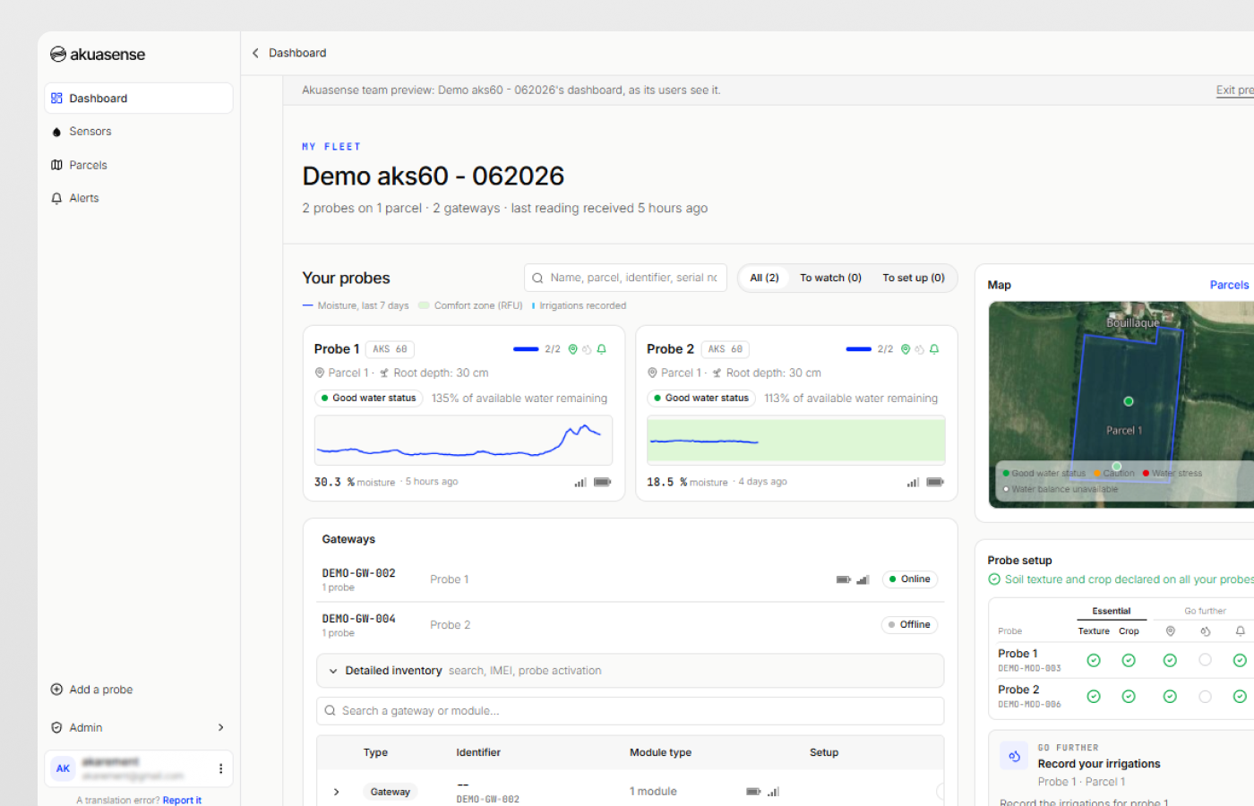
Akuasense probes measure soil moisture and temperature every 15 cm, once an hour. Their measuring principle is explained in the article Capacitive Soil Moisture Sensor: How it Works, and where to place them in the probe positioning guide. From these measurements and the characterisation of the soil, the hub calculates RAW and shows the water status of each probe. It estimates the water held by each horizon from its texture, using the Saxton and Rawls equations, and applies the crop coefficients updated in 2021. The decision to irrigate remains with the farmer, who knows the field, the crop and the water resource; the measurement gives a direct view of what is happening below the surface.

AKS connected soil moisture probe kit with 4G gateway and solar panel

Multi‑depth capacitive soil moisture probes

One capacitive sensor every 15 cm measures volumetric soil moisture and soil temperature throughout the active root zone.

3 to 9 depths depending on the model: 30, 60, 90 or 120 cm
Autonomous gateway with battery and solar panel, for up to 3 probes
Hourly 4G transmission, SIM card and data plan included
GPS position of each gateway within the plot
Designed and assembled in France

The hub: a farm's dashboard, with the water status and moisture curve of each probe, and the plot map

The hub: water monitoring for your plots

The hub centralises the readings of all your probes, on computer, tablet or smartphone.

Moisture summarised over the root zone, weighted by soil and crop, in detail by depth and as a heatmap
The water status of each probe at a glance
Soil temperature, and the battery and signal of each gateway
Soil texture by depth, crop, irrigation setup and irrigations, shown alongside the moisture curves
Plot map, built-in weather and email alerts
Your data accessible through a REST API and an MCP server

Sources

AFP (2022). “Canicule, pic et vague de chaleur, quelles différences ?” [Canicule (French term for a severe heatwave), heat peak and heatwave: what are the differences?], based on Météo-France definitions. Terre-net, 3 August 2022, updated 14 February 2024. terre-net.fr
Météo-France (2026). Bilan climatique de l'été 2026 (juin-juillet-août) [Climate report for summer 2026, June to August], 3 September 2026, and “Retour sur la 3e vague de chaleur de l'été, du 28 juillet au 19 août 2026” [Review of the third heatwave of the summer, 28 July to 19 August 2026], 31 August 2026. meteofrance.com; meteofrance.com
Arvalis (2026). “Maïs grain : comment gérer la conduite de parcelles suite à la canicule” [Grain maize: managing fields after the heatwave]. Terre-net, 3 August 2026. terre-net.fr
Allen R.G., Pereira L.S., Raes D., Smith M. (1998). Crop evapotranspiration. Guidelines for computing crop water requirements. FAO Irrigation and Drainage Paper 56, Rome. Chapters 1, 6, 7 and 8 (Tables 2, 12, 19 and 22; Equations 82 to 88). fao.org
Seger M., Curassier N., Gaillard H., Boulonne L., Boukir H., Cousin I. et al. (2022). “RU-RMQS. Bilan 2022 : évaluation du réservoir utilisable sur les sites du RMQS2” [RU-RMQS, 2022 report: assessment of available water capacity at the RMQS2 sites]. Gis Sol, INRAE, 19 May 2022. gissol.hub.inrae.fr
Chambre d'agriculture de la Drôme (2018). “Bien comprendre son sol pour valoriser sa contribution en eau” [Understanding your soil to make the most of the water it supplies]. Objectifs, no. 73. chambres-agriculture.fr
Saxton K.E., Rawls W.J. (2006). Soil water characteristic estimates by texture and organic matter for hydrologic solutions. Soil Science Society of America Journal, 70(5), 1569-1578. doi:10.2136/sssaj2005.0117
Bruand A., Duval O., Cousin I. (2004). Estimation des propriétés de rétention en eau des sols à partir de la base de données SOLHYDRO : une première proposition combinant le type d'horizon, sa texture et sa densité apparente [Estimating soil water retention properties from the SOLHYDRO database: a first proposal combining the type of horizon, its texture and its bulk density]. Étude et Gestion des Sols, 11(3), 323-332. afes.fr
Bouthier A., Scheurer O., Seger M., Lagacherie P., Beaudoin N., Deschamps T., Sauter J., Fort J.-L., Cousin I. (2022). Réservoir en eau du sol utilisable par les cultures. Guide d'estimation. [Soil water reservoir available to crops: an estimation guide]. Éditions Arvalis, Paris. sols-et-territoires.org
Tetegan M., Nicoullaud B., Baize D., Bouthier A., Cousin I. (2011). The contribution of rock fragments to the available water content of stony soils: proposition of new pedotransfer functions. Geoderma, 165(1), 40-49. doi:10.1016/j.geoderma.2011.07.001
Arvalis. “Carte des sols – Ferme de Boigneville” [Soil map of the Boigneville farm], based on Bétrémieux R., Darthout R. (1968), Étude des sols du domaine de Boigneville [Soil survey of the Boigneville farm], INRA. ecophytopic.fr
Chambre régionale d'agriculture de Poitou-Charentes, IAAT (c. 2009). Inventaire, gestion et conservation des sols (IGCS) de Poitou-Charentes : unités de sols et objectifs de rendement [Soil inventory, management and conservation (IGCS) in Poitou-Charentes: soil units and yield targets]. Gis Sol. gissol.hub.inrae.fr
Coutadeur C., Cousin I., Nicoullaud B. (2000). Influence de la phase caillouteuse sur la réserve en eau des sols. Cas des sols de Petite Beauce du Loiret [Influence of the stony phase on soil water reserves: the case of the Petite Beauce soils in the Loiret]. Étude et Gestion des Sols, 7(3), 191-205. afes.fr
Pereira L.S., Paredes P., Hunsaker D.J., López-Urrea R., Mohammadi Shad Z. (2021). Standard single and basal crop coefficients for field crops. Updates and advances to the FAO56 crop water requirements method. Agricultural Water Management, 243, 106466. doi:10.1016/j.agwat.2020.106466
Pereira L.S., Paredes P., López-Urrea R., Hunsaker D.J., Mota M., Mohammadi Shad Z. (2021). Standard single and basal crop coefficients for vegetable crops, an update of FAO56 crop water requirements approach. Agricultural Water Management, 243, 106196. doi:10.1016/j.agwat.2020.106196
Arvalis (2019). “Seule une partie de l'eau du sol est facilement exploitée par les plantes” [Only part of the soil water is readily used by plants]. Terre-net, 16 July 2019. terre-net.fr
USDA Natural Resources Conservation Service (2021). National Engineering Handbook, Part 650, Chapter 15 “Irrigation”, § 650.1505. nrcs.usda.gov
Rallo G., Paço T.A., Paredes P., Puig-Sirera À., Massai R., Provenzano G., Pereira L.S. (2021). Updated single and dual crop coefficients for tree and vine fruit crops. Agricultural Water Management, 250, 106645. doi:10.1016/j.agwat.2020.106645
Arvalis (2026). “Canicule et maïs : la météo de mi-juillet va être déterminante” [Heatwave and maize: mid-July weather will be decisive]. Terre-net, 7 July 2026. terre-net.fr
Steduto P., Hsiao T.C., Fereres E., Raes D. (2012). Crop yield response to water. FAO Irrigation and Drainage Paper 66, Rome. Chapter 2. fao.org
Brouwer C., Prins K., Heibloem M. (1989). Irrigation Water Management: Irrigation Scheduling. Training Manual no. 4. FAO, Rome. Annex I, Table 8. fao.org
Irmak S., Odhiambo L.O., Kranz W.L., Eisenhauer D.E. (2011). Irrigation Efficiency and Uniformity, and Crop Water Use Efficiency. University of Nebraska–Lincoln Extension, EC732. Table 2. extensionpubs.unl.edu
Société du Canal de Provence (2022). Conditions générales “Eaux d'irrigation agricole” [General conditions: agricultural irrigation water], in force from 1 March 2022. canaldeprovence.com
Préfecture de la Gironde (2023). Arrêté de restriction des usages de l'eau du 13 juillet 2023, annexes [Prefectoral order of 13 July 2023 restricting water use, annexes]. gironde.gouv.fr
Observatoire de l'eau du bassin de l'Adour (2009). L'irrigation dans le bassin de l'Adour. Synthèse 2009. [Irrigation in the Adour basin: 2009 summary]. eptb-a3.fr
Fereres E., Soriano M.A. (2007). Deficit irrigation for reducing agricultural water use. Journal of Experimental Botany, 58(2), 147-159. doi:10.1093/jxb/erl165
Schlegel A.J., Stone L.R., Dumler T.J., Lamm F.R. (2012). Managing diminished irrigation capacity with preseason irrigation and plant density for corn production. Transactions of the ASABE, 55(2), 525-531. k-state.edu
Nygren A., Martin D., Zoubek G., Burr C., Kranz B. (2013). “Evaluating the use of preseason irrigation”. CropWatch, University of Nebraska–Lincoln, 22 March 2013, based on Stone et al. (2008), Agronomy Journal, 100, 1185-1192. unl.edu
Lamm F.R., Klocke N.L., Rogers D.H., Stone L.R., Schlegel A.J., Aiken R.M., Shaw L.K. (2012). Assessment of plant available soil water on producer fields in Western Kansas. Proceedings of the 24th Central Plains Irrigation Conference, 37-50, based on Bordovsky and Porter (2003). k-state.edu
Kisekka I., Schlegel A., Ma L., Gowda P.H., Prasad P.V.V. (2017). Optimizing preplant irrigation for maize under limited water in the High Plains. Agricultural Water Management, 187, 154-163. Cites Musick J.T., Lamm F.R. (1990), Preplant irrigation in the Central and Southern High Plains. A review, Transactions of the ASAE, 33(6). usda.gov
Milliron L., Fulton A. (2020). “A need for winter irrigation?” Sacramento Valley Orchard Source, University of California Cooperative Extension, 3 March 2020. sacvalleyorchards.com
Wine Australia (2019). “Keep up the water during winter”, work by SARDI and CSIRO, 7 June 2019. wineaustralia.com
Bonada M., Catania A.A., Gambetta J.M., Petrie P.R. (2021). Soil water availability during spring modulates canopy growth and impacts the chemical and sensory composition of Shiraz fruit and wine. Australian Journal of Grape and Wine Research, 27(4), 491-507. doi:10.1111/ajgw.12506
Yuste J., Martínez-Porro D. (2025). Recarga hídrica antes de brotación y/o riego deficitario durante el verano: efectos agronómicos en cv. Tempranillo en la D.O. Ribera del Duero [Water recharge before budburst and/or summer deficit irrigation: agronomic effects on cv. Tempranillo in the Ribera del Duero designation of origin]. 46th OIV Congress, IVES Conference Series. ives-openscience.eu
Shackel K., Fulton A., Arnold K., Lampinen B., Milliron L. (2021). “Pulling the trigger for the start of irrigation in the spring: too much too soon for walnuts?” Sacramento Valley Orchards, University of California, 7 April 2021. sacvalleyorchards.com
Réussir (2005). “Irrigation : il faut savoir partir à point” [Irrigation: knowing when to start], advice from Arvalis-Institut du végétal, 29 June 2005. reussir.fr
Terinnov, Arvalis, Chambre d'agriculture de l'Ain (2023). Bulletin Irrigation Plaine de l'Ain [Ain plain irrigation bulletin], weeks 22–23 (2 to 8 June 2023), maize section. chambres-agriculture.fr
Moureaux B. (2021). “Comment irriguer avec des ressources en eau limitées ?” [How to irrigate with limited water resources?], with Thomas Joly (Arvalis). Perspectives Agricoles, published on Pleinchamp, 2 July 2021. pleinchamp.com
Message n° 17 – Irrigation. “Doit-on déclencher les irrigations sur céréales ?” [Should irrigation of cereals be started?]. Ouest Occitanie, April 2020. tarn.chambre-agriculture.fr
Balue M., Boutfol C. (2013). “Irriguer en viticulture – Un point sur les réglementations” [Irrigating vineyards: an update on the regulations]. Chambre d'agriculture du Var, December 2013. paca.chambres-agriculture.fr
Chambre d'agriculture du Tarn (2021). Bulletin Irrigation [Irrigation bulletin] no. 1, 16 June 2021. chambre-agriculture.fr
Chambres d'agriculture des Pays de la Loire (2023). “Optimisation irrigation” [Optimising irrigation], presentation, Rallye Cultures Bio 2023 [organic crops field day]. chambres-agriculture.fr
Chambre d'agriculture du Tarn. “Les outils d'aide au pilotage de l'irrigation : les sondes tensiométriques et capacitives” [Irrigation scheduling tools: tensiometric and capacitive probes]. chambres-agriculture.fr

Understanding soil water is a series of articles by Akuasense. Next in the series: measuring the available water of your field, reading a moisture profile at several depths, and understanding the shape of the soil volume wetted by an emitter depending on soil texture.

Should you refill the soil's available water before summer?

Three figures, one mechanism: 8 mm supplied, 10.5 mm of ETc, 24 mm of RAW

Available water capacity (TAW) and RAW: the water the soil can release to the crop

Calculating a soil’s available water capacity

Tool 1: Soil available water capacity (TAW) calculator

Your crop

Your soil, horizon by horizon

The result

Receive this simulation by email

Crop evapotranspiration (ETo, Kc and ETc)

How to calculate the irrigation capacity of a system

Tool 2: Irrigation system capacity calculator

Your system

Irrigation time

Crop requirement

Result

Set one irrigation

Receive this simulation by email

Why the soil’s remaining available water falls during a heatwave

Refilling the soil profile before summer: when is it worthwhile?

What research shows on preseason irrigation

Vines and orchards: winter, budburst or later?