Calculate the available water capacity of a soil (TAW and RAW)

Oct 22, 2026 Akuasense 21 min read

The total available water (TAW) of a soil, often called its available water capacity, is the amount of water it can release to a crop over the whole depth of its roots; it is expressed in mm of water. The calculator below lets you estimate it by entering the texture of your soil, horizon by horizon, then derives the readily available water (RAW) of your crop. The concepts it relies on are developed in the article Should you refill the soil’s available water before summer?.

Below the calculator you will find the definitions of all the technical terms it uses, together with its instructions for use.

Tool 1: Soil available water capacity (TAW) calculator

Estimate how much water your soil can supply to your crop (TAW and RAW), horizon by horizon.

Examples

Your crop

Crop

Depletion fraction p of 0.50, the value FAO cites as commonly used.

Rooting depth 60 cm
Set the rooting depth you observe in your field.
Your soil, horizon by horizon

Describe each horizon, from the surface downwards: one tab per horizon. The profile is redrawn after each change.

Available water held by each horizon

From 0 to 30 cm
Thickness 30 cm
What you know about this horizon
Stones and gravel 0%
1.95 mm of water per cm of fine earth 59 mm of water
USDA class Silt loam, Saxton and Rawls (2006)
The result

Run the simulation to calculate the result with your settings.

Total available water (TAW)
73mm of water
over 60 cm of root zone, i.e. 730 m³/ha
Readily available water (RAW)
37mm of water
depletion fraction p of 0.50 for this crop
RAW during a heatwave
22mm of water
for an ETc of 10 mm of water per day (p of 0.30)
readily available: 37 mmharder to extract: 37 mm
Without rain or irrigation, a crop with an ETc of 5 mm of water per day uses up this RAW in about 7 days.

Indicative calculation, horizon by horizon. The water held by each horizon is estimated with the equations of Saxton and Rawls¹ for a USDA texture class or a particle-size analysis, and with the values of Bruand, Duval and Cousin² for a class of the French (Aisne) texture triangle. The water held by stones follows the values used by Arvalis³. RAW is calculated with the depletion fraction p of your crop, taken from FAO-56 or from its 2021 update, or used by the hub, the web app for Akuasense connected soil moisture probes (Tables 5 and 6)^4,^5,⁶.

Terms used

mm of water: Depth of the layer of water spread over the soil surface. 1 mm of water equals 1 litre per square metre, or 10 m³ per hectare.
Horizon: Layer of soil with uniform characteristics. A soil generally consists of several horizons of different textures.
Root zone: Volume of soil in which the crop's roots are found. Its depth is the rooting depth.
Field capacity: Maximum moisture the soil retains once the drainage of water under gravity has become negligible.
Permanent wilting point: Moisture below which roots can no longer extract water from the soil.
TAW (total available water): Amount of water the soil can release to the crop: the water held between field capacity and the wilting point over the whole root zone, in mm of water. Often called the soil's available water capacity, a term also used for the water held per unit depth of soil (mm of water per cm); the Arvalis guide calls it “réservoir utilisable”.³
Transpiration: Vaporisation of the liquid water contained in plant tissues and removal of the vapour to the atmosphere, mainly through the stomata, small openings in the leaves. The plant transpires the water its roots take up from the soil; once the crop covers the soil, transpiration makes up most of its ETc.⁴
RAW (readily available water): Part of TAW that the crop uses without suffering water stress: RAW = p × TAW.
Depletion fraction p: Part of TAW the crop can use before a lack of water reduces its transpiration, that is, before water stress begins: RAW = p × TAW. With a fraction p of 0.50, the crop uses half of TAW without stress. FAO publishes it for each crop, for an ETc of 5 mm of water per day.⁴
ETo: Reference evapotranspiration: the amount of water evapotranspired in one day by a well-watered reference grass surface, calculated with the FAO Penman-Monteith method, in mm of water per day. It expresses the climate's demand for water. In France it is often called ETP (évapotranspiration potentielle, potential evapotranspiration), a term FAO discourages because it has covered different definitions and formulas.
ETc: Evapotranspiration of a crop that is not short of water, in mm of water per day.
Water stress: State of a crop that reduces its transpiration because it cannot extract enough water from the soil.
Rock fragments: Stones and gravel in a horizon, as opposed to the fine earth.

How to use the available water capacity calculator

The calculator is completed in three steps, in order: your crop, your soil, then reading the result. Each change of setting updates the soil profile diagram and the result.

1. Choose your crop and its rooting depth

Choosing your crop sets two values: the depletion fraction p and a range of rooting depths. These are the values used by the hub, the web app for Akuasense connected soil moisture probes. Fraction p comes, depending on the crop, from Table 22 of FAO-56⁴ or from its 2021 update by Pereira and colleagues^5,⁶. Rooting depth comes from the revised FAO-56 of 2025 for vegetables and field crops⁷, and from Table 22 for lucerne and grassland⁴. For trees, vines, small fruit and hops, it also depends on your irrigation method (see below).

The depletion fraction p is the part of TAW your crop can use without suffering from a lack of water. While the soil is well supplied with water, it delivers it fast enough to meet the crop’s demand, and the crop transpires normally. As the soil dries, the remaining water is held more and more tightly and reaches the roots more and more slowly. Below a threshold, it can no longer reach them fast enough to meet the transpiration demand: the crop reduces its transpiration, and water stress begins, well before the wilting point⁴. The fraction p sets this threshold: with a fraction p of 0.50, the crop can use half of TAW before stress begins. Multiplied by TAW, it gives RAW.

Rooting depth is the depth down to which the crop’s roots take up water. It depends on the species and its age, but also on the soil: a compacted horizon, bedrock or a water table stops the roots. It is best observed in a soil pit, or otherwise with an auger⁸.

FAO specifies that the upper value of the range applies to soils with no significant layering or other characteristics that restrict rooting depth, and that the lower value may be used for irrigation scheduling and the upper value for modelling water stress or for rainfed conditions⁴. Pereira and colleagues add that the lower value suits heavy soils and frequent irrigation, and the upper value light soils and longer intervals between irrigations⁵. The calculator uses the lower value, as the hub does, and shows the crop’s range.

For trees, vines, small fruit and hops, the calculator also asks for your irrigation method. FAO gives them only a maximum depth, valid in a soil with no obstacle⁴, and its 2025 revision gives them none⁷. Yet under drip irrigation, most of the roots and of the water uptake stay much higher, according to field studies and extension guides: 30 to 60 cm for most fruit trees, 60 to 100 cm for vines and almond, 90 to 150 cm for pistachio and walnut (Table 6). Some roots go deeper. If you irrigate by drip or micro-sprinkler, the calculator therefore uses this zone; with sprinklers, surface irrigation or no irrigation, it uses Table 22 of FAO-56.

If roots stop higher in your field, or go deeper, the “Set manually” button opens a slider to enter the observed depth, from 20 to 250 cm. For “Other crop”, the slider is shown straight away.

2. Describe your soil, horizon by horizon

A horizon is a layer of soil with uniform characteristics. In a soil pit, or in the cores brought up by an auger, one horizon gives way to the next when the colour, texture, structure or stone content changes. The calculator accepts up to five horizons, described from the surface downwards; each tab describes one, with its thickness.

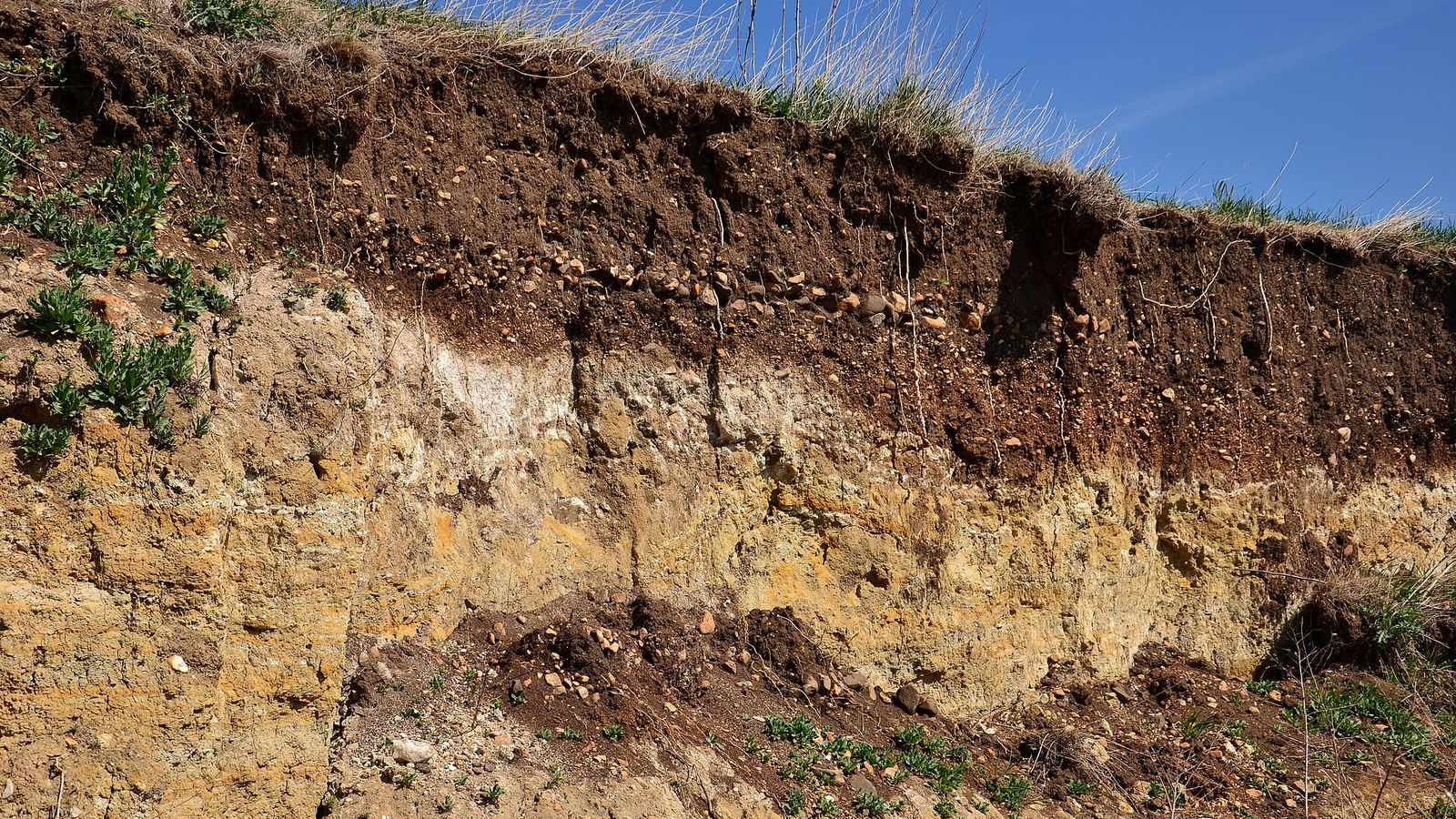
Photo: Petr Kinšt, CC BY-SA 3.0, via Wikimedia Commons, cropped.

In this photo, taken beside a road near Libědice, in the Czech Republic, the boundary between the dark brown, stony surface horizon and the pale horizon beneath it is visible to the naked eye.

For each horizon, there are three ways to enter the water it holds, from the simplest to the most precise.

Its texture. A class of the USDA texture triangle, the US classification the hub uses, with the values of Saxton and Rawls¹; or a class of the French (Aisne) texture triangle, with the values of Bruand, Duval and Cousin². The latter were measured on undisturbed soil clods, and distinguish the tilled horizon (A) from the deeper horizons (E, B or C). They do not cover calcareous horizons, and some classes have no value: the calculator flags them. The Aisne classes keep their French codes and names, as they have no official English names.
A particle-size analysis. The proportions of sand, silt and clay from the laboratory report, and the organic matter content (2.5% if the report does not give it). The calculator derives the water contents at field capacity and at the wilting point with the equations of Saxton and Rawls¹, and places the point on the USDA triangle.
Laboratory measurements. The volumetric water contents measured at field capacity (pF 2) and at the wilting point (pF 4.2), on undisturbed clods³. A laboratory often reports a gravimetric water content, in grams of water per gram of dry soil: it is converted into a volumetric water content by multiplying it by the bulk density of the soil, in g/cm³³. Example: a gravimetric water content of 22% in a soil with a bulk density of 1.4 g/cm³ corresponds to a volumetric water content of 22 × 1.4 = 30.8%.

Stones and gravel. Finally, for each horizon, the calculator asks for the share of stones and gravel, or rock fragments. They occupy part of the horizon’s volume, which therefore contains no fine earth. Their proportion is estimated by eye, with reference charts, or measured on a sample of about twenty kilograms; the two methods can give quite different results³. Arvalis considers that rock fragments can be ignored below 10% of the volume³.

Their type also matters: flint holds almost no water, whereas limestone or chalk does. The calculator applies the values used by Arvalis for each type (Table 4). For a loamy clay horizon containing 30% stones, Tetegan and colleagues calculated that ignoring this water underestimates the available water by 5% with chert and by 33% with chalk⁹.

The profile shows each horizon to scale. The blue area represents the available water it holds within the root zone, and its value in mm of water is shown in the horizon; the part of a horizon below the roots is not counted. The result gives TAW, RAW and RAW during a heatwave, explained in the next part.

The “Copy the link to this calculation” button copies a URL that contains every setting: opened in a browser, it displays the same calculation. It can be used to save a soil description or to share it with an advisor.

Format of the calculation link

The page URL accepts the following parameters, which are the same in every language:

crop: crop identifier (Tables 5 and 6), or other for a crop not listed;
root: rooting depth, in cm, a multiple of 5 from 20 to 250; if it differs from the crop’s lower value, the calculator opens the manual setting;
irrigation (optional, crops in Table 6 only): drip for drip or micro-sprinkler irrigation, the default, or other for sprinkler, surface irrigation or no irrigation;
h: one horizon, one to five of them, repeated from the surface downwards, in the form thickness,description[,stones:percentage:type], the thickness in cm, a multiple of 5 from 5 to 150, the stone percentage a multiple of 5 from 0 to 80. The description takes one of the following forms:
- usda:class, with the identifier of the USDA class (Table 2);
- aisne:code:A or aisne:code:EBC, with the code of the Aisne triangle class and the type of horizon (Table 3);
- granulo:sand-silt-clay-organic matter, in %, sand + silt + clay adding up to 100;
- labo:field capacity-wilting point, in % by volume, the first greater than the second.
The stone type is one of the identifiers in Table 4.

crop, root and h are required, and decimals use a point. An incomplete link, or one with a value outside these limits, shows the default example with a message.

Example: https://docs.akuasense.com/en/blog/available-water-capacity-calculator/?crop=grapevine-wine-grape&root=40&h=40,aisne:AL:A,stones:30:limestone describes a 40 cm clay-limestone soil with 30% limestone stones under a wine grape vineyard; the calculator shows a TAW of 50 mm of water and a RAW of 22 mm.

Interpreting the result: TAW, RAW and RAW during a heatwave

What the three figures mean

TAW is the water the soil can release to the crop over the whole root zone: the water held between field capacity and the permanent wilting point⁴. It is expressed in mm of water; 1 mm of water equals 1 litre per square metre, or 10 m³ per hectare. A TAW of 73 mm thus represents 730 m³ of water per hectare.

RAW is the part of TAW the crop extracts without reducing its transpiration. Once RAW has been used up, the remaining water is held more strongly; the crop partially closes its stomata, and water stress begins. For each crop, FAO publishes the depletion fraction p that gives RAW, valid for an ETc of 5 mm of water per day; it generally ranges from 0.30 to 0.70, and a value of 0.50 is commonly used for many crops⁴.

On the left, three magnified views of soil particles: saturated soil, field capacity and permanent wilting point. In the centre, a scale from dry soil to saturation, topped by a vine, with four thresholds: saturation, field capacity, water stress threshold and permanent wilting point. RAW runs from field capacity to the water stress threshold, TAW from field capacity to the wilting point. On the right, the corresponding states: waterlogging, no water stress, caution, water stress, unavailable water. The animation highlights each state in turn, and the vine responds: upright down to the caution zone, drooping leaves and shrivelled berries under water stress, leaves and bunch fallen to the ground below the wilting point. 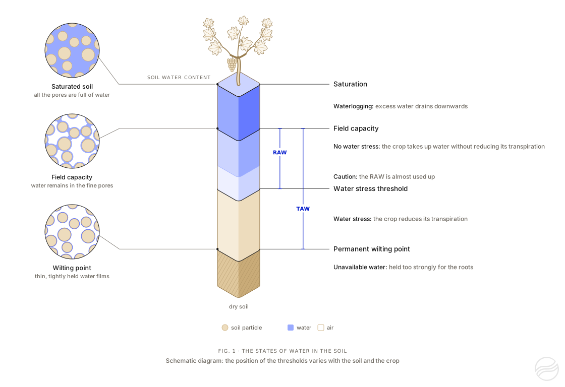— **Figure 1.** The states of water in the soil. On the left, soil particles under a magnifying glass: at saturation, water fills all the pores; at field capacity, it occupies only the finest pores; at the wilting point, only thin films remain around the particles. In the centre, the soil water content, from dry soil (beige) to saturation (blue), and the four thresholds that separate the states of water for the crop. The vine planted on top of the scale represents the crop; the animation shows how it responds to each state of the water. Schematic diagram: the position of the thresholds varies with the soil and the crop.

RAW during a heatwave takes into account that the fraction p decreases as ETc increases: the roots can no longer extract water fast enough. FAO adjusts it with the formula below, the fraction remaining between 0.1 and 0.8⁴. The calculator applies it for an ETc of 10 mm of water per day: this is the ETo recorded by Arvalis at the peak of the heatwave of late June 2026¹⁰, and the ETc of a crop whose foliage covers the ground is of the same order.

\mathrm{TAW} = \sum_{\text{horizons}} \mathrm{TAW}_h

\begin{aligned} \mathrm{TAW}_h = \bigl[\, & \mathrm{AWC}_{fe} \times (1 - \mathrm{RF}) \\ & + c \times \mathrm{RF} \,\bigr] \times d \end{aligned}

$\mathrm{TAW}_h$ : available water held by a horizon within the root zone, in mm of water

$\mathrm{AWC}_{fe}$ : available water capacity of the fine earth of the horizon, in mm of water per cm, that is $(\theta_{FC} - \theta_{WP}) \times 10$ , with the water contents in m³ of water per m³ of soil

$\mathrm{RF}$ : share of the horizon volume occupied by rock fragments (stones and gravel), from 0 to 1 (0.30 for 30%); $c$ : water held by the stones, in mm of water per cm of stones

$d$ : thickness of the horizon within the root zone, in cm

\mathrm{RAW} = p \times \mathrm{TAW}

p_{\text{heat}} = p + 0.04 \times (5 - \mathrm{ETc})

example: a 30 cm silt loam horizon over a 30 cm sand horizon, without stones, holds $1.95 \times 30 + 0.49 \times 30 = 73$ mm of water; with $p = 0.50$ , RAW is 37 mm; for an ETc of 10 mm of water per day, $p_{\text{heat}} = 0.30$ and RAW falls to 22 mm

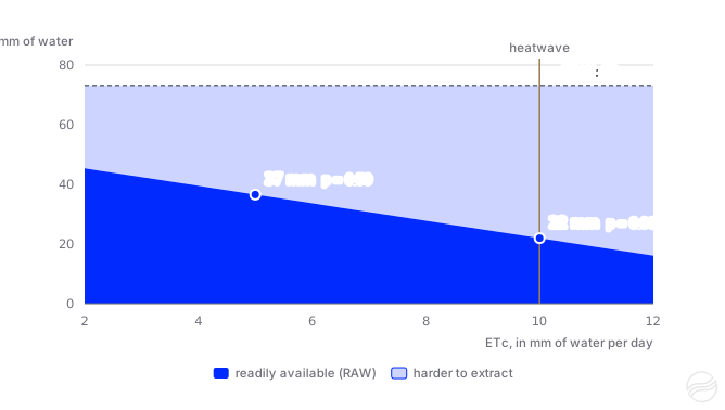
RAW as a function of ETc for a TAW of 73 mm of water: 37 mm for an ETc of 5 mm of water per day (p of 0.50); 22 mm for an ETc of 10 mm of water per day (p of 0.30). — **Figure 2.** RAW as a function of ETc, for the TAW of the example: 73 mm of water, silt loam over sand, depletion fraction of 0.50. Adjusted with the FAO formula⁴, the fraction p goes from 0.50 for an ETc of 5 mm of water per day to 0.30 for 10 mm: RAW falls from 37 to 22 mm of water, and it is used up in about 2 days instead of 7.

What the result can be used for

Estimating how many days RAW lasts. Without rain or irrigation, a full RAW lasts, as a first approximation, a number of days equal to RAW divided by ETc: 37 mm of water for an ETc of 5 mm of water per day lasts about 7 days. This period shortens quickly as ETc rises, since RAW decreases at the same time: for an ETc of 10 mm of water per day, the 22 mm of RAW in the example lasts about 2 days (Figure 2).
Putting an irrigation application in context. FAO specifies that the net depth of an irrigation should be smaller than or equal to the root zone depletion, and that water applied above field capacity drains below the roots⁴. On a root zone whose RAW has just been used up, a net application larger than RAW, 37 mm in the example, therefore exceeds field capacity. With drip irrigation, only part of the soil surface is wetted, around 30 to 40% according to FAO⁴: the water is spread over a smaller volume of soil, and this calculation does not apply as it stands.
Comparing. Two horizons, two fields, two rooting depths: the calculator shows which horizon holds the most water, and how much TAW changes when roots reach a few centimetres deeper or shallower.

Putting the result in context

For a uniform horizon without stones, the available water per cm of soil depends first on texture: around 0.5 to 1.1 mm of water per cm for a sand, and 1.3 to 1.9 mm for a loam or a silt loam, according to the water contents published in FAO-56⁴ (Table 1).

Over a real profile, TAW also depends on the depth the roots explore and on the stones: it is much lower as soon as a calcareous horizon or bedrock stops the roots close to the surface, or when stones are abundant. Two examples from France:

Boigneville (Essonne), Arvalis experimental farm. The TAW of a clay-limestone soil (French argilo-calcaire) whose top 40 cm lie on a highly calcareous horizon is around 55 mm of water; that of a neighbouring clay loam, where hard limestone appears only below 120 cm, is around 120 mm¹¹.
Poitou-Charentes. The regional soil reference system uses 60 to 80 mm of water for shallow groie soils and 110 to 130 mm for deep groies, classes of that reference system¹².

Table 1. Orders of magnitude of TAW according to texture

Horizon texture (USDA class)	mm of water per cm of soil	TAW over 30 cm (mm of water)	over 60 cm	over 90 cm
Sand	0.5–1.1	15–33	30–66	45–99
Sandy loam	1.1–1.5	33–45	66–90	99–135
Loam, silt loam	1.3–1.9	39–57	78–114	117–171
Clay	1.2–2.0	36–60	72–120	108–180

Horizon of uniform texture, without stones. Values calculated from the water contents at field capacity and at the wilting point published in FAO-56 (Table 19)⁴, whose US texture classification does not exactly match the triangle used in France. The Saxton and Rawls equations, which the hub uses, give 1.95 mm of water per cm for the typical composition of a silt loam (Table 2), slightly above the FAO range. Both are estimates from the texture class alone, with an error of around 0.5 mm per cm (see “Accuracy and limitations”).

Accuracy and limitations

The result is an order of magnitude, for four reasons.

A texture class covers a range of soils. For French soils, the root mean square error of an available water capacity estimated from the texture class alone is 0.047 to 0.058 cm³ of water per cm³ of soil, that is 0.47 to 0.58 mm of water per cm¹³. Over a 60 cm horizon, this represents around 30 mm of water. Within a single class of the Aisne triangle, the standard deviation of the available water capacity ranges from 0.15 to 0.50 mm of water per cm, because of differences in soil structure².
Two definitions of field capacity coexist. Saxton and Rawls set it at a tension of 33 kPa¹, the French references at 10 kPa (pF 2)². For the same soil, the latter gives a higher field capacity, and therefore a larger available water capacity: for a sand, 0.49 mm of water per cm with the USDA classes, compared with 0.60 to 0.73 mm with the Aisne triangle (Tables 2 and 3).
Rooting depth matters as much as texture. In a uniform soil, TAW is proportional to it: using 80 cm instead of 60 cm increases it by a third.
Stones and compaction change the water held. The calculator accounts for stones according to their type, but not for compaction, which only a measurement captures.

Methods based on local measurements are the most precise³: water contents measured in the laboratory on each horizon, or monitoring soil moisture at several depths, which shows the water the crop actually uses.

The values used by the calculator

The calculator uses only the values below and the formulas on this page: the same calculation can be done by hand.

Table 2. USDA texture classes: water contents and water held

USDA texture class	Identifier	θ at field capacity (% vol.)	θ at wilting point (% vol.)	mm of water per cm
Sand	`sand`	9.9	5.0	0.49
Loamy sand	`loamy-sand`	13.2	6.8	0.63
Sandy loam	`sandy-loam`	18.7	9.2	0.95
Loam	`loam`	26.9	12.6	1.43
Silt loam	`silt-loam`	30.5	11.0	1.95
Silt	`silt`	31.1	5.8	2.53
Sandy clay loam	`sandy-clay-loam`	27.8	17.7	1.01
Clay loam	`clay-loam`	35.7	21.8	1.39
Silty clay loam	`silty-clay-loam`	37.9	21.0	1.69
Sandy clay	`sandy-clay`	37.7	26.6	1.11
Silty clay	`silty-clay`	41.6	27.7	1.39
Clay	`clay`	45.1	34.0	1.11

Water contents calculated with the equations of Saxton and Rawls¹ for the typical composition of each class and 2.5% organic matter, at 33 kPa (field capacity) and 1,500 kPa (wilting point); these are the hub’s values. Loam is a texture balanced between sand, silt and clay; silt is a much finer texture.

Table 3. Classes of the French (Aisne) texture triangle: water held by the fine earth

Code	Aisne triangle class	Tilled horizon (A), mm of water per cm	Deeper horizons (E, B, C), mm of water per cm
`ALO`	Argile lourde	1.24	1.12
`AL`	Argile limoneuse	1.36	1.13
`A`	Argile	—	0.93
`AS`	Argile sableuse	1.73	0.95
`LA`	Limon argileux	1.73	1.49
`LAS`	Limon argilo-sableux	1.67	1.48
`LSA`	Limon sablo-argileux	1.43	1.27
`LM`	Limon moyen	2.13	2.07
`LMS`	Limon moyen sableux	1.83	1.96
`LL`	Limon léger	—	—
`LLS`	Limon léger sableux	—	—
`LS`	Limon sableux	1.62	—
`SA`	Sable argileux	1.28	1.03
`SL`	Sable limoneux	1.31	1.16
`S`	Sable	0.60	0.73

Values of Bruand, Duval and Cousin, established on non-calcareous or slightly calcareous horizons, between pF 2 and pF 4.2²; a dash marks a class without a reference value. Class names are kept in French, for want of official English names.

Table 4. Water held by stones according to their type

Stone type	Identifier	mm of water per cm of stones
Inert (hold no water)	`inert`	0.00
Flint	`flint`	0.18
Chert	`chert`	0.55
Limestone	`limestone`	0.97
Gaize	`gaize`	1.91
Chalk	`chalk`	2.28

Values used by Arvalis³.

Table 5. Depletion fraction p and rooting depth: vegetables, field crops and grassland

Crop	Identifier	Fraction p	Depth (cm)	Source of fraction p
Other crop	`other`	0.50	—	FAO-56 (commonly used fraction p)
Aerobic rice	`aerobic-rice`	0.35	100	Pereira et al., 2021 (field crops)
Artichoke	`artichoke`	0.45	60–120	Pereira et al., 2021 (vegetables)
Asparagus	`asparagus`	0.45	120–180	Pereira et al., 2021 (vegetables)
Aubergine	`eggplant`	0.45	40–100	Pereira et al., 2021 (vegetables)
Beetroot	`table-beet`	0.45	45–100	Pereira et al., 2021 (vegetables)
Broccoli	`broccoli`	0.40	40–90	Pereira et al., 2021 (vegetables)
Brussels sprouts	`brussels-sprouts`	0.40	40–90	Pereira et al., 2021 (vegetables)
Bulb onion	`bulb-onion`	0.30	30–60	FAO-56
Cabbage	`cabbage`	0.40	30–50	Pereira et al., 2021 (vegetables)
Carrot	`carrot`	0.30	30–50	Pereira et al., 2021 (vegetables)
Castor bean	`castor-bean`	0.60	80–130	Pereira et al., 2021 (field crops)
Cauliflower	`cauliflower`	0.40	40–90	Pereira et al., 2021 (vegetables)
Chickpea	`chickpea`	0.45	70–100	Pereira et al., 2021 (field crops)
Chilli pepper	`chili-pepper`	0.30	50–120	Pereira et al., 2021 (vegetables)
Cotton	`cotton`	0.60	100–170	Pereira et al., 2021 (field crops)
Courgette	`zucchini`	0.50	60–110	Pereira et al., 2021 (vegetables)
Cowpea	`cowpea`	0.45	60–130	Pereira et al., 2021 (field crops)
Cucumber	`cucumber`	0.40	60–120	Pereira et al., 2021 (vegetables)
Dry bean	`dry-bean`	0.45	50–90	Pereira et al., 2021 (field crops)
Durum wheat	`durum-wheat`	0.55	100–150	Hub (no row in FAO-56)
Faba bean	`faba-bean`	0.45	50–70	Pereira et al., 2021 (field crops)
Field pea	`field-pea`	0.45	60–100	Pereira et al., 2021 (field crops)
Flax	`flax`	0.50	100–150	Pereira et al., 2021 (field crops)
Fodder beet	`fodder-beet`	0.55	70–120	Hub: values for sugar beet
Forage sorghum	`forage-sorghum`	0.55	100–150	Pereira et al., 2021 (field crops)
French bean	`green-bean`	0.45	50–90	FAO-56
Garlic	`garlic`	0.30	30–50	Pereira et al., 2021 (vegetables)
Grain maize	`grain-maize`	0.50	60–150	Pereira et al., 2021 (field crops)
Grain sorghum	`grain-sorghum`	0.55	100–150	Pereira et al., 2021 (field crops)
Groundnut	`groundnut`	0.50	50–100	Pereira et al., 2021 (field crops)
Lentil	`lentil`	0.50	60–80	Pereira et al., 2021 (field crops)
Lettuce	`lettuce`	0.30	30–50	FAO-56
Lucerne (1st cut)	`alfalfa-1st-cut`	0.55	100–200	FAO-56
Melon	`melon`	0.40	60–120	Pereira et al., 2021 (vegetables)
Oats	`oats`	0.55	100–150	Pereira et al., 2021 (field crops)
Oilseed rape	`oilseed-rape`	0.50	80–130	Pereira et al., 2021 (field crops)
Parsnip	`parsnip`	0.40	50–100	Pereira et al., 2021 (vegetables)
Pearl millet	`pearl-millet`	0.55	100–200	Pereira et al., 2021 (field crops)
Perennial ryegrass (cutting)	`perennial-ryegrass-cutting`	0.60	60–100	FAO-56, “Rye Grass hay” row
Perennial ryegrass (grazing)	`perennial-ryegrass`	0.60	50–150	FAO-56, “Grazing Pasture — Rotated Grazing” row
Perennial ryegrass (turf)	`perennial-ryegrass-turf`	0.40	50–100	FAO-56, “Turf grass — cool season” row
Potato	`potato`	0.40	40–60	Pereira et al., 2021 (vegetables)
Radish	`radish`	0.30	30–50	Pereira et al., 2021 (vegetables)
Rye	`rye`	0.55	60–120	Pereira et al., 2021 (field crops)
Safflower	`safflower`	0.60	100–200	Pereira et al., 2021 (field crops)
Sesame	`sesame`	0.60	100–150	Pereira et al., 2021 (field crops)
Silage maize	`silage-maize`	0.50	60–150	Pereira et al., 2021 (field crops)
Soya bean	`soybean`	0.50	60–140	Pereira et al., 2021 (field crops)
Spinach	`spinach`	0.20	30–50	Pereira et al., 2021 (vegetables)
Spring wheat	`spring-wheat`	0.55	100–150	Pereira et al., 2021 (field crops)
Strawberry	`strawberry`	0.25	30–50	Pereira et al., 2021 (vegetables)
Sugar beet	`sugar-beet`	0.55	70–120	FAO-56
Sunflower	`sunflower`	0.45	80–200	Pereira et al., 2021 (field crops)
Sweet pepper	`sweet-pepper`	0.30	50–100	FAO-56
Sweet potato	`sweet-potato`	0.40	100–120	Pereira et al., 2021 (vegetables)
Sweetcorn	`sweet-corn`	0.50	60–150	Pereira et al., 2021 (field crops)
Temporary grassland	`temporary-grassland`	0.60	60–100	FAO-56
Tomato (open field)	`tomato-open-field`	0.40	60–120	Pereira et al., 2021 (vegetables)
Turnip	`turnip`	0.50	50–90	Pereira et al., 2021 (vegetables)
Watermelon	`watermelon`	0.40	80–150	Pereira et al., 2021 (vegetables)
Winter barley	`winter-barley`	0.55	60–120	Pereira et al., 2021 (field crops)
Winter squash	`winter-squash`	0.40	90–150	Pereira et al., 2021 (vegetables)
Winter wheat	`winter-wheat`	0.55	100–150	Hub

Values used by the hub: depletion fraction p valid for an ETc of 5 mm of water per day, and range of rooting depths. Fraction p comes from Table 22 of FAO-56⁴ or from its 2021 update by Pereira and colleagues, for field crops⁵ and for vegetables⁶. Rooting depth comes from the revised FAO-56 of 2025 (Tables 6.1 and 6.2)⁷, except for lucerne and grassland, which these tables do not give: they keep Table 22 of FAO-56⁴. Fodder beet, absent from both, takes the depths of sugar beet. The calculator uses the lower value of the range, which FAO indicates may be used for irrigation scheduling⁴. For three crops, marked “Hub”, fraction p is a value used by the hub.

Table 6. Depletion fraction p and rooting depth: trees, vines, small fruit and hops

Crop	Identifier	Fraction p	Drip (cm)	Other irrigation (cm)	Sources
Almond	`almond`	0.40	60–100	100–200	^14,¹⁵
Apple	`apple`	0.50	40–90	100–200	^16,¹⁷
Apricot	`apricot`	0.50	30–80	100–200	¹⁸
Avocado	`avocado`	0.70	30–60	50–100	¹⁹
Cherry	`cherry`	0.50	50–100	100–200	²⁰
Clementine	`clementine`	0.50	30–60	120–150	^21,²²
Fig	`fig`	0.65	60–90	120–170	²³
Gold kiwifruit	`gold-kiwifruit`	0.35	40–60	70–130	²⁴
Grapevine (table grape)	`grapevine-table-grape`	0.35	60–100	100–200	²⁵
Grapevine (wine grape)	`grapevine-wine-grape`	0.45	60–100	100–200	²⁵
Hazelnut	`hazelnut`	0.40	40–60	100–200	²⁶
Highbush blueberry	`highbush-blueberry`	0.50	30–50	60–120	²⁷
Hop	`hop`	0.50	60–100	100–120	²⁸
Lemon	`lemon`	0.50	30–60	120–150	^21,²²
Olive	`olive`	0.65	60–100	120–170	^29,^30,³¹
Orange	`orange`	0.50	30–60	120–150	^21,²²
Peach	`peach`	0.50	40–80	100–200	^32,³³
Pear	`pear`	0.50	30–90	100–200	³⁴
Persimmon	`persimmon`	0.50	50–60	100–200	³⁵
Pistachio	`pistachio`	0.40	90–120	100–150	³⁶
Plum	`plum`	0.50	30–80	100–200	¹⁸
Pomegranate	`pomegranate`	0.65	60	120–170	^37,³⁸
Walnut	`walnut`	0.50	90–150	170–240	³⁹

Values used by the hub: depletion fraction p valid for an ETc of 5 mm of water per day, taken from Table 22 of FAO-56⁴. “Drip”: the depth that holds most of the roots and of the water uptake of a mature orchard under drip or micro-sprinkler irrigation, according to the sources shown; the lower value applies to the usual case, the upper value to a light or deep soil, and some roots go deeper. For pistachio and walnut, these values come from extension guides, as no measurements under drip irrigation exist. “Other irrigation”: maximum depth in Table 22 of FAO-56, for a soil with no obstacle⁴. Absent from this table, hazelnut takes the values of almond, persimmon those of apple, and fig and pomegranate those of olive, for fraction p as well as for depth. The calculator uses the lower value of the range.

Saxton and Rawls (2006) equations used for a particle-size analysis

S = sand (%) / 100        C = clay (%) / 100        OM = organic matter (%)

θ1500t = 0.031 - 0.024 S + 0.487 C + 0.006 OM + 0.005 S×OM - 0.013 C×OM + 0.068 S×C
θWP    = θ1500t + (0.14 θ1500t - 0.02)                     wilting point (1,500 kPa)

θ33t   = 0.299 - 0.251 S + 0.195 C + 0.011 OM + 0.006 S×OM - 0.027 C×OM + 0.452 S×C
θFC    = θ33t + (1.283 θ33t² - 0.374 θ33t - 0.015)          field capacity (33 kPa)

mm of water per cm of fine earth = (θFC - θWP) × 10         water contents in m³ per m³

Equations taken from Saxton and Rawls¹, with organic matter in %, as in the hub. The USDA class of the point is given by the USDA texture triangle.

Table 7. Calculator examples and results

Example	Horizons	Crop, rooting depth	TAW (mm of water)	RAW (mm of water)	RAW during a heatwave (mm of water)
Silt loam over sand	30 cm of silt loam (USDA) over 30 cm of sand (USDA)	Other crop (p of 0.50), 60 cm	73	37	22
Clay-limestone soil, 40 cm	40 cm of argile limoneuse (Aisne AL, tilled horizon), 30% limestone stones	Wine grape (p of 0.45), 40 cm	50	22	12
Limon moyen (Aisne), 120 cm	30 cm of limon moyen (Aisne LM, tilled horizon) over 90 cm of limon moyen (deeper horizon)	Grain maize (p of 0.50), 120 cm	250	125	75

These calculations in the hub

The hub performs the same calculation for each probe, and compares it with the measurement. In the probe settings, the soil texture is declared at each measurement depth, as a USDA class or from a particle-size analysis, organic matter included; the hub derives the water held with the equations of Saxton and Rawls. The declared crop sets the depletion fraction p and the rooting depth, with the same values as in this calculator, and a cap can limit this depth when an obstacle stops the roots higher up.

The hub then calculates TAW and RAW for the root zone (“Total reserve” and “Readily available” in its interface) and, from the soil moisture measured every hour at each depth, the root zone depletion, the share of available water remaining and the water status of the probe.

The calculator on this page goes further on four points:

stones, according to their type;
the Aisne triangle references;
laboratory measurements;
RAW during a heatwave.

Measurement shows what calculation can only estimate:

the depth reached by an irrigation or by rain;
the horizons in which the roots take up water;
the rate at which soil moisture falls.

Akuasense connected multi-depth soil moisture probes, from €135 excl. VAT, measure soil moisture and temperature every 15 cm, once an hour; their measuring principle is explained in the article Capacitive Soil Moisture Sensor: How it Works. The hub brings these measurements together. The decision to irrigate remains with the farmer, who knows the field, the crop and the water resource.

Akuasense professional connected soil moisture probes are available from €135 excl. VAT.

AKS connected soil moisture probe kit with 4G gateway and solar panel

Multi‑depth capacitive soil moisture probes

One capacitive sensor every 15 cm measures volumetric soil moisture and soil temperature throughout the active root zone.

3 to 9 depths depending on the model: 30, 60, 90 or 120 cm
Autonomous gateway with battery and solar panel, for up to 3 probes
Hourly 4G transmission, SIM card and data plan included
GPS position of each gateway within the plot
Designed and assembled in France

The hub: a farm's dashboard, with the water status and moisture curve of each probe, and the plot map

The hub: water monitoring for your plots

The hub centralises the readings of all your probes, on computer, tablet or smartphone.

Moisture summarised over the root zone, weighted by soil and crop, in detail by depth and as a heatmap
The water status of each probe at a glance
Soil temperature, and the battery and signal of each gateway
Soil texture by depth, crop, irrigation setup and irrigations, shown alongside the moisture curves
Plot map, built-in weather and email alerts
Your data accessible through a REST API and an MCP server

Sources

Saxton K.E., Rawls W.J. (2006). Soil water characteristic estimates by texture and organic matter for hydrologic solutions. Soil Science Society of America Journal, 70(5), 1569-1578. doi:10.2136/sssaj2005.0117
Bruand A., Duval O., Cousin I. (2004). Estimation des propriétés de rétention en eau des sols à partir de la base de données SOLHYDRO : une première proposition combinant le type d'horizon, sa texture et sa densité apparente [Estimating soil water retention properties from the SOLHYDRO database: a first proposal combining the type of horizon, its texture and its bulk density]. Étude et Gestion des Sols, 11(3), 323-332. afes.fr
Bouthier A., Scheurer O., Seger M., Lagacherie P., Beaudoin N., Deschamps T., Sauter J., Fort J.-L., Cousin I. (2022). Réservoir en eau du sol utilisable par les cultures. Guide d'estimation. [Soil water reservoir available to crops: an estimation guide]. Éditions Arvalis, Paris. sols-et-territoires.org
Allen R.G., Pereira L.S., Raes D., Smith M. (1998). Crop evapotranspiration. Guidelines for computing crop water requirements. FAO Irrigation and Drainage Paper 56, Rome. Chapters 7 and 8 (Tables 19, 20 and 22; Equations 82 to 84). fao.org
Pereira L.S., Paredes P., Hunsaker D.J., López-Urrea R., Mohammadi Shad Z. (2021). Standard single and basal crop coefficients for field crops. Updates and advances to the FAO56 crop water requirements method. Agricultural Water Management, 243, 106466. doi:10.1016/j.agwat.2020.106466
Pereira L.S., Paredes P., López-Urrea R., Hunsaker D.J., Mota M., Mohammadi Shad Z. (2021). Standard single and basal crop coefficients for vegetable crops, an update of FAO56 crop water requirements approach. Agricultural Water Management, 243, 106196. doi:10.1016/j.agwat.2020.106196
Pereira L.S., Allen R.G., Paredes P., López-Urrea R., Raes D., Smith M., Kilic A., Salman M. (2025). Crop evapotranspiration. Guidelines for computing crop water requirements. Second edition, revised 2025. FAO Irrigation and Drainage Paper 56 Rev.1. FAO, Rome. Tables 6.1 and 6.2 (rooting depths). doi:10.4060/cd6621en
Agriculture Victoria (2025). “Determining readily available water”, fact sheet, updated 22 September 2026. agriculture.vic.gov.au
Tetegan M., Nicoullaud B., Baize D., Bouthier A., Cousin I. (2011). The contribution of rock fragments to the available water content of stony soils: proposition of new pedotransfer functions. Geoderma, 165(1), 40-49. doi:10.1016/j.geoderma.2011.07.001
Arvalis (2026). “Maïs grain : comment gérer la conduite de parcelles suite à la canicule” [Grain maize: managing fields after the heatwave]. Terre-net, 3 August 2026. terre-net.fr
Arvalis. “Carte des sols – Ferme de Boigneville” [Soil map of the Boigneville farm], based on Bétrémieux R., Darthout R. (1968), Étude des sols du domaine de Boigneville [Soil survey of the Boigneville farm], INRA. ecophytopic.fr
Chambre régionale d'agriculture de Poitou-Charentes, IAAT (c. 2009). Inventaire, gestion et conservation des sols (IGCS) de Poitou-Charentes : unités de sols et objectifs de rendement [Soil inventory, management and conservation (IGCS) in Poitou-Charentes: soil units and yield targets]. Gis Sol. gissol.hub.inrae.fr
Roman Dobarco M., Cousin I., Le Bas C., Martin M. (2019). Pedotransfer functions for predicting available water capacity in French soils, their applicability domain and associated uncertainty. Geoderma, 336, 81-95. doi:10.1016/j.geoderma.2018.08.022
Andreu L., Hopmans J.W., Schwankl L.J. (1997). Spatial and temporal distribution of soil water balance for a drip-irrigated almond tree. Agricultural Water Management, 35(1-2), 123-146. doi:10.1016/S0378-3774(97)00018-8
Brown P., Hopmans J., Olivos A., Sanden B. Determination of root distribution, dynamics, phenology and physiology of almonds to optimize fertigation practices. Final report, FREP 11-0461-SA. California Department of Food and Agriculture. cdfa.ca.gov
Svoboda P., Haberle J., Moulik M., Raimanová I., Kurešová G., Mészáros M. (2023). The effect of drip irrigation on the length and distribution of apple tree roots. Horticulturae, 9(3), 405. doi:10.3390/horticulturae9030405
Kadayıfçı A., Şenyiğit U., Dağdelen N., Öz H., Atılgan A. (2010). The effects of different irrigation methods on root distribution, intensity and effective root depth of young dwarf apple trees. African Journal of Biotechnology, 9(27), 4217-4224. core.ac.uk
Paltineanu C., Nicolae S., Tanasescu N., Chitu E., Ancu S. (2017). Investigating root density of plum and apple trees grafted on low-vigor rootstocks to improve orchard management. Erwerbs-Obstbau, 59(1), 29-37. doi:10.1007/s10341-016-0293-7
Kalmar D., Lahav E. (1977). Water requirements of avocado in Israel. I. Tree and soil parameters. Australian Journal of Agricultural Research, 28(5), 859-868. doi:10.1071/AR9770859
Li P., Tan H., Wang J., Cao X., Yang P. (2019). Evaluation of water uptake and root distribution of cherry trees under different irrigation methods. Water, 11(3), 495. doi:10.3390/w11030495
Cassiani G., Boaga J., Vanella D., Perri M.T., Consoli S. (2015). Monitoring and modelling of soil-plant interactions: the joint use of ERT, sap flow and eddy covariance data to characterize the volume of an orange tree root zone. Hydrology and Earth System Sciences, 19(5), 2213-2225. doi:10.5194/hess-19-2213-2015
Vanella D., Ramírez-Cuesta J.M., Sacco A., Longo-Minnolo G., Cirelli G.L., Consoli S. (2021). Electrical resistivity imaging for monitoring soil water motion patterns under different drip irrigation scenarios. Irrigation Science, 39(1), 145-157. doi:10.1007/s00271-020-00699-8
Abdolahipour M., Kamgar-Haghighi A.A., Sepaskhah A.R., Zand-Parsa S., Honar T. (2020). Root length density of rainfed fig trees under different times, amounts, and positions of supplemental irrigation. Journal of Agricultural Science and Technology, 22(4), 1137-1150. modares.ac.ir
Calabritto M., Mininni A.N., Di Biase R., Pietrafesa A., Dichio B. (2024). Spatio-temporal dynamics of root water uptake and identification of soil moisture thresholds for precision irrigation in a Mediterranean yellow-fleshed kiwifruit orchard. Frontiers in Plant Science, 15, 1472093. doi:10.3389/fpls.2024.1472093
Smart D.R., Schwass E., Lakso A., Morano L. (2006). Grapevine rooting patterns: a comprehensive analysis and a review. American Journal of Enology and Viticulture, 57(1), 89-104. doi:10.5344/ajev.2006.57.1.89
Olsen J.L. (2013). Growing Hazelnuts in the Pacific Northwest: Orchard Site Selection. EM 9076. Oregon State University Extension Service. oregonstate.edu
Bryla D.R. (2011). Crop evapotranspiration and irrigation scheduling in blueberry. Gerosa G. (ed.), Evapotranspiration – From Measurements to Agricultural and Environmental Applications, InTech. doi:10.5772/18311
Stampfl J., Fuß S., Münsterer J., Portner J., Schlagenhaufer A. (2021). Tropfbewässerung und Fertigation bei Hopfen. LfL-Information. Bayerische Landesanstalt für Landwirtschaft. lfl.bayern.de
Searles P.S., Saravia D.A., Rousseaux M.C. (2009). Root length density and soil water distribution in drip-irrigated olive orchards in Argentina under arid conditions. Crop & Pasture Science, 60(3), 280-288. doi:10.1071/CP08135
Fernández J.E., Moreno F., Cabrera F., Arrue J.L., Martín-Aranda J. (1991). Drip irrigation, soil characteristics and the root distribution and root activity of olive trees. Plant and Soil, 133(2), 239-251. doi:10.1007/BF00009196
Gómez-del-Campo M. (2013). Summer deficit-irrigation strategies in a hedgerow olive orchard cv. 'Arbequina': effect on fruit characteristics and yield. Irrigation Science, 31(3), 259-269. doi:10.1007/s00271-011-0299-8
Bryla D.R., Dickson E., Shenk R., Johnson R.S., Crisosto C.H., Trout T.J. (2005). Influence of irrigation method and scheduling on patterns of soil and tree water status and its relation to yield and fruit quality in peach. HortScience, 40(7), 2118-2124. doi:10.21273/HORTSCI.40.7.2118
Conesa M.R., Conejero W., Vera J., Ruiz-Sánchez M.C. (2023). Assessment of trunk microtensiometer as a novel biosensor to continuously monitor plant water status in nectarine trees. Frontiers in Plant Science, 14, 1123045. doi:10.3389/fpls.2023.1123045
Janssens P., Diels J., Vanderborght J., et al. (2015). Numerical calculation of soil water potential in an irrigated 'conference' pear orchard. Agricultural Water Management, 148, 113-122. doi:10.1016/j.agwat.2014.09.023
Porras-Jorge R., Aguilar J.M., Baixauli C., Pascual B., Pascual-Seva N. (2025). Effect of deficit irrigation on agronomic and physiological performance of young persimmon (Diospyros kaki Thunb.) trees. Agronomy, 15(7), 1671. doi:10.3390/agronomy15071671
Culumber M., Zaccaria D. (2021). 2021 Pistachio Irrigation: Mitigation Strategies for Drought. University of California Cooperative Extension. ucanr.edu
Buesa I., Badal E., Guerra D., et al. (2012). Development of an irrigation scheduling recommendation for pomegranate trees (Punica granatum). Options Méditerranéennes, Série A, 103, 141-145, CIHEAM. ciheam.org
Hiwale S.S., More T.A., Bagle B.G. (2011). Root distribution pattern in pomegranate 'Ganesh' (Punica granatum L.). Acta Horticulturae, 890, 323-326. doi:10.17660/ActaHortic.2011.890.44
Beede R.H., Fulton A.E. Irrigation Scheduling for Walnuts. University of California Cooperative Extension. ucanr.edu

This calculator comes from the article Should you refill the soil’s available water before summer?, which offers three other tools: an irrigation capacity calculator, a wetted depth calculator and a seasonal soil water balance simulator.

Calculate the available water capacity of a soil (TAW and RAW)

Tool 1: Soil available water capacity (TAW) calculator

1Your crop

2Your soil, horizon by horizon

3The result

Receive this simulation by email